In this post I’m going to attempt to give an intuitive introduction to Fisher Information, (very briefly) Jeffrey priors, and the lower bounds on the variance of unbiased estimators i.e. the Cramer-Rao bound. Hopefully this post will be shorter than my last couple…

Resources

• Fisher Information & Efficiency - Robert L. Wolpert
• Fisher Information - Wikipedia
• The Fisher Information (video) - Mutual Information (YouTube Channel)
• A Tutorial on Fisher Information - Alexander Ly, Maarten Marsman, Josine Verhagen, Raoul Grasman and Eric-Jan Wagenmakers (All University of Amsterdam)
• Stat 5102 Notes: Fisher Information and Confidence Intervals Using Maximum Likelihood - Charles J. Geyer
• The Fisher Information - Gregory Gunderson
• De Bruijn’s Identity: Theory & Applications - Emergent Mind
• Generalization of the de Bruijn’s identity to general φ-entropies and φ-Fisher informations - Irene Valero Toranzo, Steeve Zozor and Jean-Marc Brossier
• Information Geometry - Wikipedia
• Fisher information metric - Wikipedia
• An Elementary Introduction to Information Geometry - Frank Nielson
• Some inequalities satisfied by the quantities of information of Fisher and Shannon - A.J. Stam
• Relations between Kullback-Leibler distance and Fisher information - Anand G. Dabak & Don H. Johnson
• THEORETICAL NEUROSCIENCE I \(\Vert\) Lecture 16: Fisher information - Prof. Jochen Braun
• THE FORMAL DEFINITION OF REFERENCE PRIORS

Table of Contents

• Information and Fisher Information
• Example Cases of Fisher Information values
  • Normal
  • Poisson
  • Laplace
  • Cauchy
• Fisher Information Derivation From Relative Entropy
• Uninformative (Jeffreys) priors and the Fisher information
  • Example Cases of Uninformative (Jeffreys) priors
  • Limitations of the Jeffreys prior
• Cramer-Rao Bound
• Summary/Conclusion

Definition of the Fisher Information

Fisher information is a fundamental quantity used across statistics to quantify and describe information on parameters given our models and data.

In more rigorous terms,

“In mathematical statistics, the Fisher information is a way of measuring the amount of information that an observable random variable X carries about an unknown parameter \(\theta\) of a distribution that models X.” - Wikipedia

But I’m presuming that if you’ve clicked on this post either that the above definition doesn’t make sense to you, or your a nerd who enjoys learning about statistics, so I’ll skip the motivation for this post and jump straight into trying to understand it.

I’m first going to try and approach this purely by interpretting the definition at face value and then do a more fundamental derivation after we know what’s going on. The Fisher Information is defined as,

But honestly this is just a little to esoteric for me to internalise. So I’m gonna make some pretty pictures.

Below is a GIF with three rows and two columns.

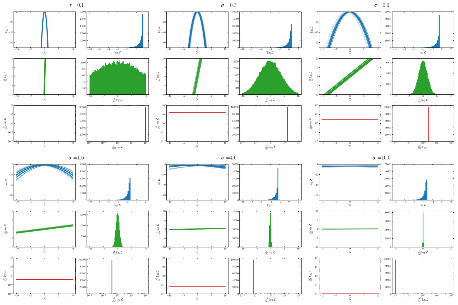
The first column exemplifies what some transformations of normal distribution looks like with respect to the random variable it describes, with a mean of 0 and varying standard deviation values. It specifically show the log, the derivative of the log-likelihood with respect to a parameter of interest (the mean) known as the score, and the second derivative of the log-likelihood with respect to this parameter.

The right column are histograms of these same values with random samples taken from the given likelihood (kind like Monte Carlo error propagation for nonlinear functions).

The definition of the Fisher information, boils down to the variance of the second row second column distribution or equivalently the negative of the expected value of the bottom right. Which annoyingly for the normal distribution is always the same value so there isn’t really a ‘distribution’¹

Okay, but what does this actually imply about our models? Well notice that as the log-likelihood distribution broadens, the variance in the distribution of the score becomes smaller. Or in a different way of looking at it, the number of extreme derivative values decreases. Or a different way again, it’s the expected value of the magnitude of the derivatives squared, more higher magnitude values, more info.

If what we’re interested in is information (which makes sense as we’re trying to understand Fisher information) then this narrowing the score distribution, indicates that our data is becoming less informative about what the true value of the parameter we’re interested in is. If we have large gradients, then our likelihood is telling us very strongly what direction the true value is in, while for small gradients it only weakly tells us. And if the variance is small, then more of our values congregate towards zero/smaller values.

I’ll now bash out an FAQ style answer to “But why this?” in regards to why we specifically construct the Fisher information in this manner:

• Question: By why is expected value for the score is always zero?
  • Answer: See below.
• Question: By why the variance in the log-derivative instead of expected value?

  • Answer: The expected value for the score is always zero, which doesn’t relate different amounts of information for different sets of parameters. Mathematically this can be seen as, for the general case for parameter \(\theta\) and likelihood/probability distribution \(\mathcal{L}(x\vert\theta)\),

    \[\begin{align} &\mathbb{E}_{x\sim \mathcal{L}(x|\theta)}\left[\frac{\partial}{\partial \theta} \log \mathcal{L}(x|\theta)\right] \\ &= \int_x \mathcal{L}(x|\theta) \frac{\partial}{\partial \theta} \log \mathcal{L}(x|\theta) dx \\ &= \int_x \mathcal{L}(x|\theta) \frac{1}{\mathcal{L}(x|\theta)} \frac{\partial}{\partial \theta} \mathcal{L}(x|\theta) dx \\ &= \int_x \frac{\partial}{\partial \theta} \mathcal{L}(x|\theta) dx \\ &= \frac{\partial}{\partial \theta} \int_x \mathcal{L}(x|\theta) dx \\ &= \frac{\partial}{\partial \theta} 1 \\ &= 0 \\ \end{align}\]

  • Answer 2: The average here will always relate back to in some way the derivative at the mode of the distribution/the true value. Which should have a maximal likelihood value and hence should be at least a local max. At this point we shouldn’t get any directional information because we shouldn’t move, but this looks equivalent to having no information where we don’t know where to move.

• Question: By how is the variance of the derivative equivalent to the negative of the expected value of the second?

  • Answer: Again, a tinsy bit of math (using the above fact to simplify \(\text{Var}[X] = \mathbb{E}[X^2] - (\mathbb{E}[X])^2 = \mathbb{E}[X^2]\))

    \[\begin{align} &-\mathbb{E}\left[\frac{\partial^2}{\partial \theta^2} \log \mathcal{L}(x|\theta) \right] \\ &= -\mathbb{E}\left[\frac{\partial}{\partial \theta} \frac{\frac{\partial}{\partial \theta} \mathcal{L}(x|\theta)}{\mathcal{L}(x|\theta)}\right] \\ &= -\mathbb{E}\left[\frac{\frac{\partial^2}{\partial \theta^2} \mathcal{L}(x|\theta)}{\mathcal{L}(x|\theta)} - \left(\frac{\frac{\partial}{\partial \theta} \mathcal{L}(x|\theta)}{\mathcal{L}(x|\theta)}\right)^2\right] \\ &= -\mathbb{E}\left[\frac{\frac{\partial^2}{\partial \theta^2} \mathcal{L}(x|\theta)}{\mathcal{L}(x|\theta)}\right] + \mathbb{E}\left[\left(\frac{\frac{\partial}{\partial \theta} \mathcal{L}(x|\theta)}{\mathcal{L}(x|\theta)}\right)^2\right] \\ &= 0 + \mathbb{E}\left[\left(\log \frac{\partial}{\partial \theta} \mathcal{L}(x|\theta)\right)^2\right] \\ &= \text{Var}\left[ \log \frac{\partial}{\partial \theta} \mathcal{L}(x|\theta)\right] \\ \end{align}\]
• Question: By why do this with the log-likelihood, why not just the likelihood?
  • Answer: In part because it’s nicer to compute. The derivatives propagate linearly in the case of the log-likelihood, but in the case of the likelihood you would have truncated products for example. Plus some more fundamental reasons that I’ll touch on in the more fundamental derivation. The fundamental derivation is just by looking at the problem with different initial conditions though, you probably could come up with some similar alternative formulation using just the likelihood, but then we’d go back to the first point on tractability.

Now, before we jump into what is in my opinion the nicer way to understand the Fisher information (through entropy) let’s look at how we can actually calculate the Fisher information analytically for some distributions.

Example Cases of Fisher Information values

For all of these, try and have a go yourself first and I’ll be doing it for the same parameters that I do so for in the GIFs (coz I needed to do this to make them anyways).

Normal

Poisson

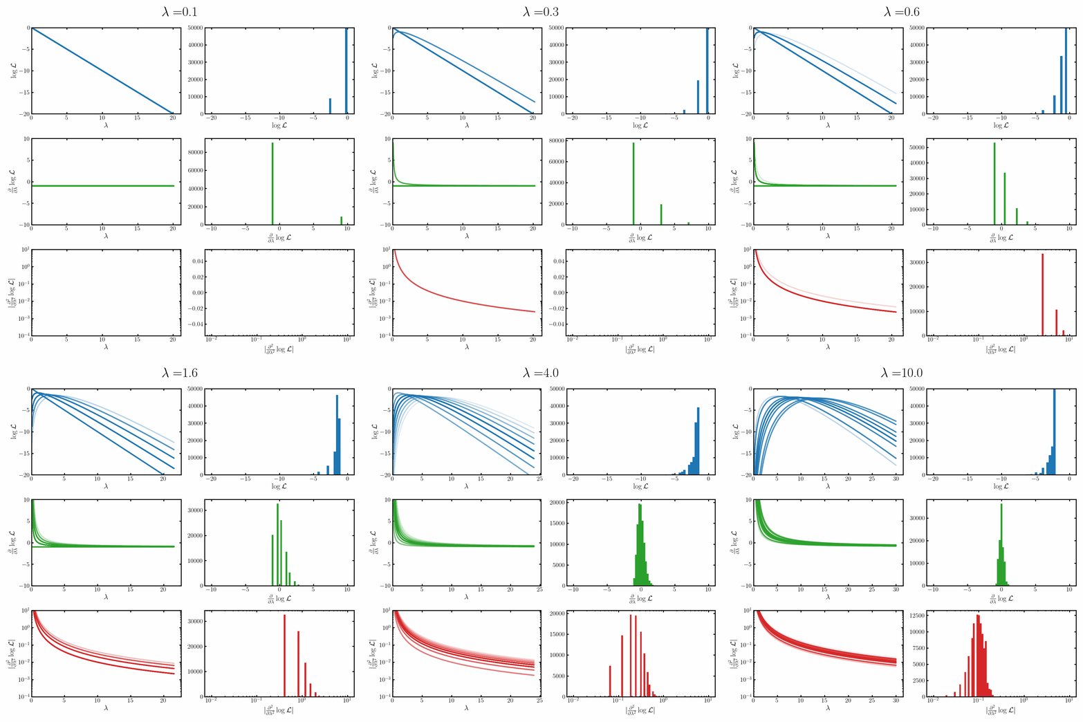
Laplace

For this one we’ll be using the first derivative definition as the Laplace doesn’t satisfy some required smoothness constraints.

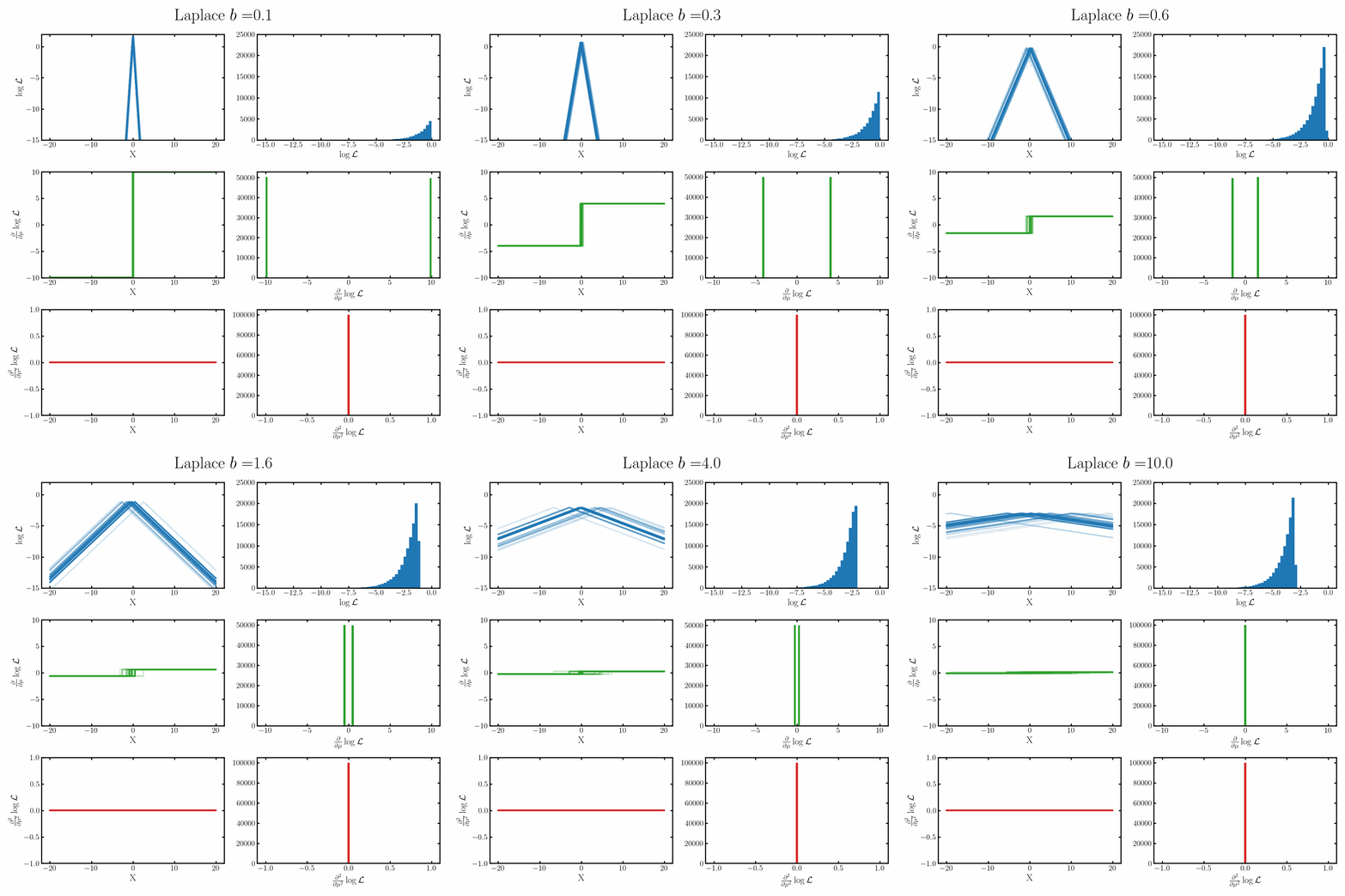
Cauchy

For this one we’ll be using the second derivative definition as it’s slightly easier to get the integral result. But it is a little harder I think because it’s not an exponential family.

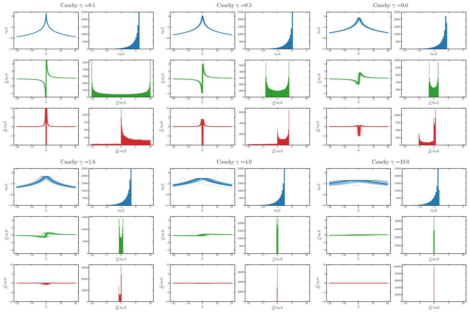
Fisher Information Derivation From Relative Entropy

Now for this very in-depth derivation, I’m going to presume you know what entropy is, and how it works from a statistical stand-point. If you are unfamiliar with the Entropy I’d recommend the following resources:

• Entropy (for data science) Clearly Explained!!! - StatQuest with Josh Starmer
• And of course I quite like Steve Mould’s “one line” definition of entropy, except he does it in many more than one line… A better description of entropy -Steve Mould
• And if you want something that isn’t a video then Three tutorial lectures on entropy and counting - David Galvin is pretty to the point with basic concepts and pretty exhaustive when it comes to it’s further properties

If you wanna skip that, or have a quick refresher, to quote Gavlin,

“…, it is most helpful to (informally) think of entropy as a measure of the expected amount of surprise evinced by a realization of X, or as a measure of the degree of randomness of X.” - David Galvin in the work Three tutorial lectures on entropy and counting

With the mathematical definition of (specifically conditional) entropy for a random variable \(X\) can be given by the following.

The typical example being flipping a coin. We have max entropy or ‘randomness’ if it is a fair coin, it is truly random whether we’ll get a heads or a tails. You can calculate the entropy of this as \(H(X) \approx 0.693\).

While if we have an unfair coin, where the heads is 99 times more probable than the tails, then the result isn’t nearly as random and you can be pretty confident in saying that the result of any single toss will be a heads. You can calculate the entropy of this example as \(H(X) \approx 0.056\).

In the second example we can also imagine that if we did get a tails, then that would add a lot of ‘information’ in that maybe the coin is more fair than we thought. Or in another way, if our system isn’t truly random, we can say certain things about different outcomes or we have more ‘potential’ information.

e.g. If we are using light to look at a star. If the photons coming at us were truly random, we could never say anything about the star, as they have nothing to do with it, they’re random. But if they are completely deterministic, the photons the star emits and we receive are exactly the same, and have no randomness, then we can say quite a lot about the star.

Relative entropy, more well known as the KL Divergence, denoted something like \(\text{KL}(P\Vert Q)\).

If \(H(P)\) is the “true” entropy with \(H(P, Q\vert\theta) = -\int_X P(X\vert\theta) \log Q(x\vert\theta) dx\) is the “cross entropy” (the surprise of \(Q\) measured by \(P\)) then the KL divergence or relative entropy can be expressed as \(\text{KL}(P \Vert Q) = H(P, Q\vert\theta) - H(P\vert \theta)\).

You can think about it as how much extra information would be accessible if one used the ‘right’ distribution \(P\) instead of \(Q\) or equivalently how much information is lost if we incorrectly use \(Q\) instead of \(P\).

Using the continuous version of the definition we can find that the Fisher Information is given as the second derivative or Hessian of the KL divergence between the true distribution, assuming the likelihood for a true value of \(\theta\) and an approximate value given by a sample/datapoint. Informally I’d say it’s like asking how sensitive the relative information between the true distribution and a given sample are i.e. the curvature of the KL divergence with respect to the parameter of interest.

This is very easy to see through a taylor expansion of the cross entropy about the difference between the distribution using the true value \(\theta\) and the approximate value \(\theta^* = \theta + \epsilon\) .

Moving the first term over to the otherside we can see the KL divergence pop out and that the second term will vanish as it’s the average of the score which we established to be 0 above. This leaves us with,

i.e. if we take the second derivative term in our taylor expansion, or more simply, take the second derivative (where by first principles we take \(\epsilon \rightarrow 0\)) we find that

In summary, the Hessian of the infinitesimal form of the KL divergence gives the fisher information. Note that this doesn’t equate to the second derivative of the entropy is the Fisher information, although it’s frustratingly close. The closest expression for that is the following, and the second term doesn’t vanish in general.

Although sometimes the Fisher information as the negative hessian of the entropy, such as when we look at the mean of the normal distribution and I think the location parameters for distributions in the location-scale family. And there’s something called De Bruijn’s identity which I can’t seem to find the assumptions for.

In summary, you can think of the interpretation of the pull between the true distribution and our approximate as another reason why we have the log -likelihood in our definition of Fisher information.

Uninformative (Jeffreys) priors and the Fisher information

The key thing that Jeffreys priors try to be a non-informative prior that nicely transforms under reparameterisation. One example of this kind of prior, or the example, is the Jeffreys prior given as,

But why? What ‘niceness’ does this encode?

The Problem

Well let’s do an example, Alex and Casey are betting on some unfair/weighted coin flips and both trying to optimally calculate the probability of getting heads, \(p_H\), to maximise their profits, as one does. Additionally they want to look at the odds \(\psi_H = \frac{p_H}{1-p_H} = \frac{p_H}{p_T}\) for some other calculations they need to make optimal bets.

They both don’t want to bias any results so both assume what they think are uninformative priors: uniform priors.

Alex thinks that a uniform prior on the probabilities is appropriate. This means that their posterior for \(k\) flips follows,

Casey instead wants to look at the odds and thinks they should put a uniform prior on the odds. Their posterior then ends up being,

If we want to see how Alex’s system looks from Casey’s “odds” perspective, we can then look at how each of these assumptions translate into the other parameterisation.

The Jacobian for the transformation is:

Alex’s posterior transformed to odds:

They disagree! Even though they both claimed to be “uninformative,” the act of being flat in one space created a “hidden” bias in the other.

Alex’s prior implies that extreme odds are very unlikely, while Casey’s prior would imply that high probabilities are much more likely than low ones.

This is one of the reasons that Bayesian perspectives on probability can be quite nice, as the explicit need to quantify assumptions through the priors means that you don’t implicitly set the prior to a uniform distribution and get the kerfuffle above.

The Solution: Jeffreys Prior

Now, let’s use the Jeffreys prior \(p(\theta) \propto \sqrt{\mathcal{I}(\theta)}\).

For the Bernoulli (coin flip) likelihood:

In \(p_Η\) - space:

In \(\psi_Η\) - space:

Let’s see if Alex and Casey agree now. If Alex uses the Jeffreys prior for \(p_H\) and transforms it to \(\psi_H\):

So if you transform the prior that Alex assumed for their model, you would get the prior that Casey assumed in their model!

So the “niceness” of the Jeffreys prior is coordinate independence. By using the square root of the Fisher Information, we ensure that:

• Prior Invariance: The prior itself accounts for the “stretching” of the parameter space.Posterior
• Consistency: Alex and Casey can work in whatever units they want (probability, odds, log-odds) and they will always arrive at the same physical conclusion.
• Information Symmetry: The prior puts equal weight on equal amounts of “distinguishable information” rather than equal intervals of a coordinate ruler.

In essence, the Jeffreys prior interprets the parameter space as a manifold where the Fisher Information is the metric. The \(\sqrt{\mathcal{I}(\theta)}\) is the “volume element” of that manifold, making the prior a uniform distribution over the geometry of the likelihood rather than the numbers on the axis.

But like … why?

But, why does the square root of the fisher information even work? Or make sense? Well you can interpret the Fisher info as a magnifying glass for how we perceive changes in a system.

1. The “Dense” Region (High Information)

A large \(I(\theta)\) means the “distance”² between the distribution \(\mathcal{L}(x\vert\theta)\) and \(\mathcal{L}(x\vert\theta + \epsilon)\) is huge even for a tinsy \(\epsilon\).

Because the distribution changes so quickly, the data is sensitive to the parameter. It is easy to tell the difference between \(\theta = 0.50\) and \(\theta = 0.51\).

As a result your estimates will have a low variance because the data clearly “points” to the true parameter value.

2. The “Sparse” Region (Low Information)

A small \(I(\theta)\) means the distribution \(\mathcal{L}(x\vert\theta)\) is almost identical to \(\mathcal{L}(x\vert\theta + \epsilon)\). They overlap almost perfectly.

The data is “blind” to the parameter here. Whether the true \(\theta\) is \(0.5\) or \(0.7\), the outcomes you observe look roughly the same.

So your estimates will have high variance or you can think of it as the “information” being spread thin. You need more data to distinguish between nearby estimates of \(\theta\).

How does this relate to the priors?

If a region is “dense” (large \(I(\theta)\)), a single unit of \(\theta\) (say, from 0.5 to 0.6) actually contains more distinguishable “states” of the world than a unit in a sparse region.

Uniform Priors ignore this; they give the same “weight” to the 0.5–0.6 interval regardless of how much the distributions actually change. e.g. if you assume a uniform prior you load the prior with the same amount of information in areas that you would gain little information to areas where you would get a lot.

Jeffreys Priors use \(\sqrt{I(\theta)}\) to “stretch” the prior mass in dense regions and “compress” it in sparse regions.

By doing this, you aren’t being “flat” over the numbers (which are arbitrary), you are being “flat” over the observable differences in the model.

This is why Jeffreys is often called a “representation-independent” prior—it cares about the statistical impact of the parameter!

(If this still doesn’t make click well for you I’m gonna do some GIFs below and maybe that’ll work better.)

Example Cases of Uninformative (Jeffreys) priors

Now I won’t show the priors for the mean/median values for the above distributions coz they’re all uniform with respect to the actual parameter, i.e. they’re all flat priors to begin with, which is kind of interesting but not interesting to look at. I’ll instead look at the Jeffreys priors on the scale parameters as those at least have ‘shapes’ but also to look at the priors on the kind of ‘natural’ parameters for these likelihoods where the information is distributed evenly/what coordinate system of the parameter space gives you a uniform prior.

Normal

The natural parameter here is \(\log(\sigma)\) and the fisher info for \(\sigma\) is \(2/\sigma^2\).

Laplace

The natural parameter here is \(\log(b)\) and the fisher info for \(b\) is \(1/b^2\).

Poisson

The natural parameter here is \(\sqrt{\lambda}\) and the fisher info for \(\lambda\) is \(1/\lambda\).

Cauchy

The natural parameter here is \(\log{\gamma}\) and the fisher info for \(\gamma\) is \(1/2\gamma^2\).

Limitations of the Jeffreys prior

Now I’ve made this sound great and all, but some issues come up in high-dimensional spaces, where they often fail to be “non-informative” and can lead to pathological conclusions/results.

In multiparameter problems, the Jeffreys prior is defined as the square root of the determinant of the Fisher Information Matrix, \(\begin{align} p(\boldsymbol{\theta}) \propto \sqrt{\det \mathcal{I}(\boldsymbol{\theta})}. \end{align}\)

Because this approach treats all parameters as a joint geometric block, it can accidentally introduce dependencies or “hidden” information that biases the marginal estimates.

An example is just the Normal distribution with unknown mean \(\mu\) and variance \(\sigma^2\). The Jeffreys prior for this case is \(p(\mu, \sigma) \propto \sigma^{-2}\) (which you can see above). Using this leads to marginal inferences that are less efficient than those derived from the Reference Prior \(p(\mu, \sigma) \propto \sigma^{-1}\).

In high dimensions, the volume of the information manifold can grow in a way that “pushes” the posterior mass toward extreme values, violating the very spirit of ignorance Jeffreys sought to capture³.

There’s also some weird philosophical stuff with basing the Jeffreys prior strictly on the likelihood. Because \(\mathcal{I}(\theta) = \mathbb{E}_{x\sim \mathcal{L}(x\vert\theta)} [ (\frac{\partial}{\partial \theta} \log \mathcal{L}(x\vert\theta))^2 ]\), the prior is calculated based on the expectation over the sample space—meaning can depend on the experimental design (the “stopping rule”) rather than just the observed data.

Jeffreys priors are focused on geometric invariance (making the prior look the same in any coordinate system), but more often now the average statistician focuses on information maximization. This leads to the concept of the “Reference Prior”, defined as the prior that maximizes the expected “missing information” about a parameter. Or more formally, it maximizes the Kullback-Leibler divergence between the prior and the posterior as the number of data points \(n \to \infty\).

Nicely, in single-parameter models, the Reference Prior and the Jeffreys Prior are identical. So it’s quite common in multi-parameter setups to use a product of single parameter Jeffreys priors. For a quick intro on reference priors I’d recommend An introduction to reference priors (video) by Ben Lambert.

Lower bounds on the variance of unbiased estimators (Cramer-Rao bound)

In any real-world work we are interested in how much information we can get out of a given system, and often we would like to have an estimate of how much before we spend a billion dollars. The Cramer-Rao bound is one way of estimating a lower bound of the variance of a given quantity (presuming our model is correct).

Let’s say you have some variable \(\hat{\theta}=u(X)\) that is an unbiased estimate of \(\theta\) where \(X\sim \mathcal{L}(x\vert\theta)\). Which we can describe as,

Then to make the math a lil’ easier, I’m gonna denote \(\partial_\theta \log \mathcal{L}(x\vert\theta) = \ell(x\vert\theta)\) such that the above can be represented as,

Then we’ll use the following,

\(\mathbb{E}\left[\ell(X \vert \theta)\right]=0\) as derived above, so ,

Then through the Cauchy Schwarz inequality or more simply through the fact that the correlation is less than or equal to 1, then,

In plain-ish english, this says that the variance of any estimate of \(\theta\) can only be as low as the reciprocal of the Fisher information. Or more plainly again the precision of an estimate on \(\theta\) can only be as good as the Fisher information.

You can see that limit is satisfied (the inequality is an equality) for the normal, laplace and Poisson distributions above⁴.

If you want the multivariate version of the proof/derivation then this video by Mike, the Mathematician is very good.

Summary/Conclusion

The Fisher Information and it’s multivariate version the Fisher Information matrix have widespread uses and underpin many statistical and machine learning methods. Hopefully, this post has elucidated where some of its properties come from, and if not, maybe one of the resources I link at the top of the post will be useful.

Footnotes