
Image Classification and Molecular Structure Reconstruction with Constant Curvature VAEs
Published:
In this post, I’ll go through Constant Curvature VAEs (traditional, hyperspherical, and hyperbolic) for image data classification and molecular structure reconstruction.
Table of Contents
- Variational Autoencoder Recap: Coolness and Limitations
- A sneak peek at Hyperspherical VAEs
- Hyperspherical VAE
- Hyperbolic VAE
- Image Classification and Generation with MNIST and LFW
- Molecular Structure Reconstruction with QM9
- Conclusions
Prerequisites
- Strong foundation of multivariable calc, linear algebra, and nerdiness
General Resources
- Directional Statistics
- Data Compression and generation with Variational Autoencoders
- Hyperspherical VAE - Nicola De Cao Blog Post
- GitHub Repo for Hyperspherical VAE implementation
Papers
- An Introduction to Variational Autoencoders
- Hyperspherical Variational Auto-Encoders - Davidson et al. 2022
- Main reference for hyperspherical VAEs
- Continuous Hierarchical Representations with Poincaré Variational Auto-Encoders
- Main reference for hyperbolic VAEs
- Geometric deep learning: going beyond Euclidean data - Bronstein et al. 2017
- Directional Statistics-based Deep Metric Learning for Image Classification and Retrieval
- Mixed-Curvature Variational Autoencoders - Skopek et al. 2020
- Quantum chemistry structures and properties of 134 kilo molecules - QM9 dataset
- ToensorFlow - QM9 Dataset
Also going to try something different in this post and actually link some sources for some broader statements in a reference section1, which will basically just be the authors, titles, and link to the given source. I’ll continue just having a basic link for definitional and to-the-point stuff.
Variational Autoencoder Recap: Coolness and Limitations
(If you’re already very familiar with VAEs you can skip this section and just move to the hyperspherical example.)
The key property of variational autoencoders [1, 2] is that they reduce dimensionality like standard autoencoders but do so in a more regularised manner. Learning a conditional gaussian distribution in the latent space/bottleneck layer rather than single point estimates which lead to enhanced performance and more regularised latent spaces among many other benefits [3].
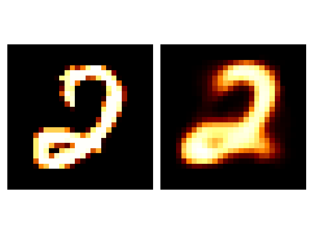
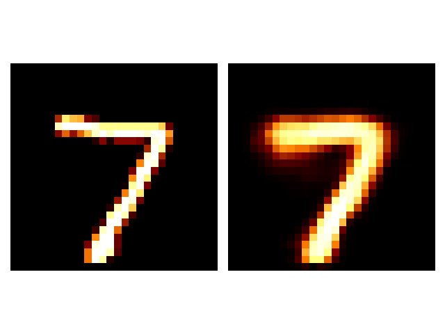
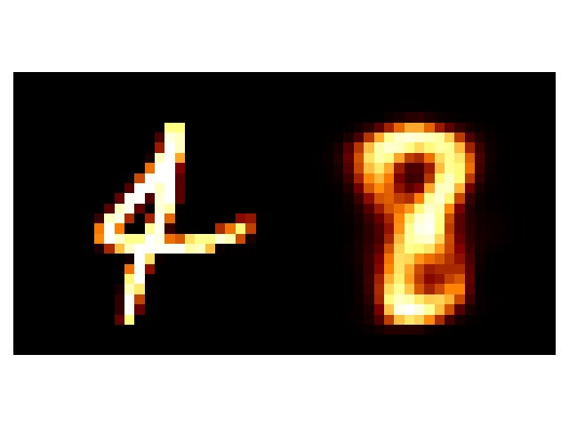
One easy and common way to do this is with the MNIST dataset that contains roughly 70,000 handwritten 28x28 pixelated digits in black and white. Some examples I put below.

A VAE (or standard autoencoder) is then constructed to take in this data, learn a conditional gaussian on a latent dimensional space 2 (or some point estimate in the lower dimensional space) and then uses this lower dimensional representation to reproduce the data. This process for autoencoders.
First the Autoencoder takes in the data, \(\vec{x}_i\), uses an encoder to transform this into some coordinate in a lower dimensional space, \(\vec{z}_i\), and then the decoder uses \(\vec{z}_i\) to try and reproduce \(\vec{x}_i\) denoted here with \(\vec{y}_i\).

The Variational Autoencoder takes in the data, \(\vec{x}_i\), uses an encoder to transform it into a mean and standard deviation describing a normal distribution over \(\vec{z}\), and then we sample a given \(\vec{z}_i\) (utilising the reparameterization trick ) to try and produce a normal distribution over \(\vec{x}\) with the decoder, with a given sample denoted here as \(\vec{y}_i\) (and it is almost always assumed that \(\vec{y}_i = \vec{\mu}_i\), the mean of the data space distribution).

(If you want more details on VAEs I’d recommend any of the sources I linked above or my own post that goes through it in much more detail.)
Using the code from my previous post on VAEs we can put the AE and VAE constructions side-by-side with the real data and also look at where the data is mapping to in the 2D latent space I constructed.
First we’ll have a look at the standard autoencoder reconstructions and latent space.
First thing we can notice is that it completely messed up the 4, and the digits are typically more blurry than their true counterparts (although this is typical in shallow neural network image construction across different architectures). Then we look at the latent space.
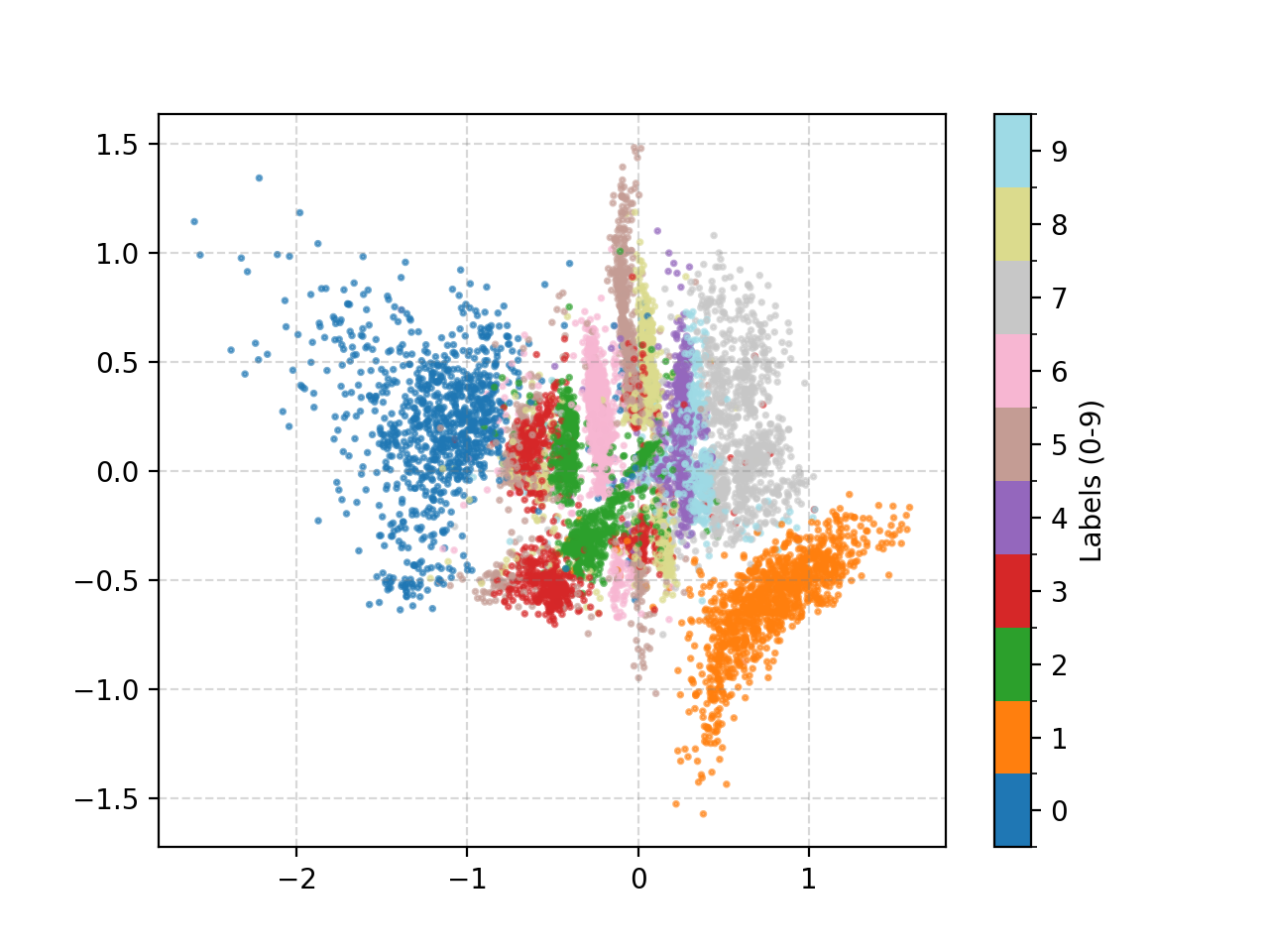
In a word: messy. There’s some slightly strange behaviours induced because I enforced the samples to fall between 0 and 1 for plot-ability, but the distribution of 4, 7, and 9 are overlapping and separated. Many of the individual distributions also have weird parts that are spread out across the space for some reason. that doesn’t really indicate that the VAE is considering them part of the same label set as we would expect.
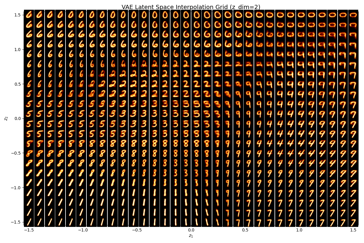
If we uniformly grid this space and see what the decoder tries to reconstruct we can also kind of see how the VAE is interpretting the space.
We can see that some areas are very clearly defined and others not so much. And even more annoyingly, if we tried to interpolate between some pretty reasonable numbers (that look similar) like 8 and 9 then we can cross through regions that are completely uninterpretable and carry zero meaning (lower left corrner). And the transitions between numbers that the VAE decides are similar also contain weird artefacts (like the transition between 4 and 6, or the region between 2, 5 and 8).
Now let’s compare the above with VAEs.
Overall, a little better. The 4 doesn’t transform to a 4 this time but to an 8, but at least it’s a number. And the groups in the latent space seem to have more intelligible structure to them. And the transformation of the latent space still has a region with some unintelligible digits (the very centre) but the transitions and distributions altogether look better.
The indistinguishability in the centre is actually pretty typical in low latent dimensional VAEs as the prior on the distributions is centred at 0 so the groups are pulled in this direction. If you wanted to get rid of this you would need to use some uncentred/uninformative prior, but that only really gives us the uniform distribution, which won’t regularise our space.
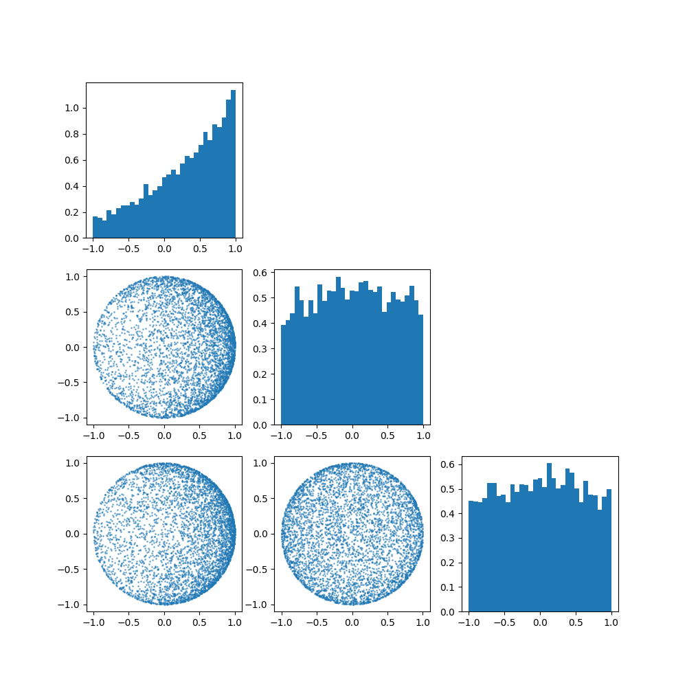
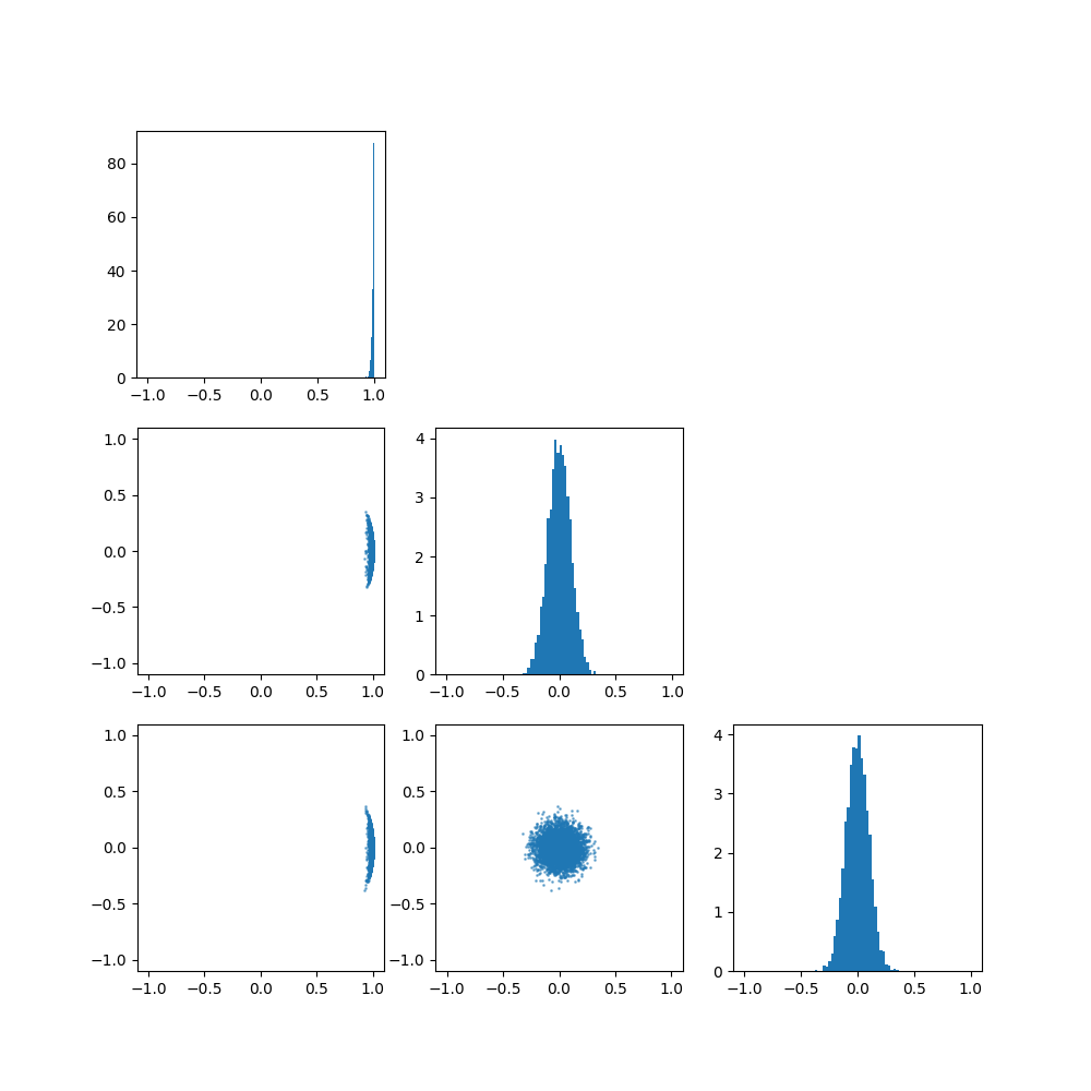
And it turns out for high dimensional VAEs, samples from the normal distribution really start to look like uniform samples on the sphere (the so called ‘soap bubble effect’). e.g. For the two plots below, which one do you think is a set of samples from a high dimensional normal distribution, and which is from a high dimensional sphere? (And I assure you there is in fact one of each here.)


Not any easy game is it?
This leads us to try and think of geometries where the centralising effect is mitigated or even removed, and maybe waste less time sampling a sphere indirectly and instead just sample the sphere itself! And this also motivates looking at other geometrical spaces and whether they can inherently better represent some data structures.
A sneak peek at Hyperspherical VAEs
In this section I want to show a little of why we are interested in mixed curavture VAEs by looking at the above MNIST example with a hyperspherical (example of constant curvature) VAE.
The basic idea is that the normal distribution priors used in the standard VAE above have a tendency to pull representations towards 0. This is true for all the clusters of datapoints and thus inherently they are pulled together and often overlap quite significantly in this region.
And although we want a smooth representation, we also would like a clear one. As we move within the latent space there are obvious regions that are a ‘3’, an ‘8’ and a ‘1’ with some boundary that nicely transitions between them.
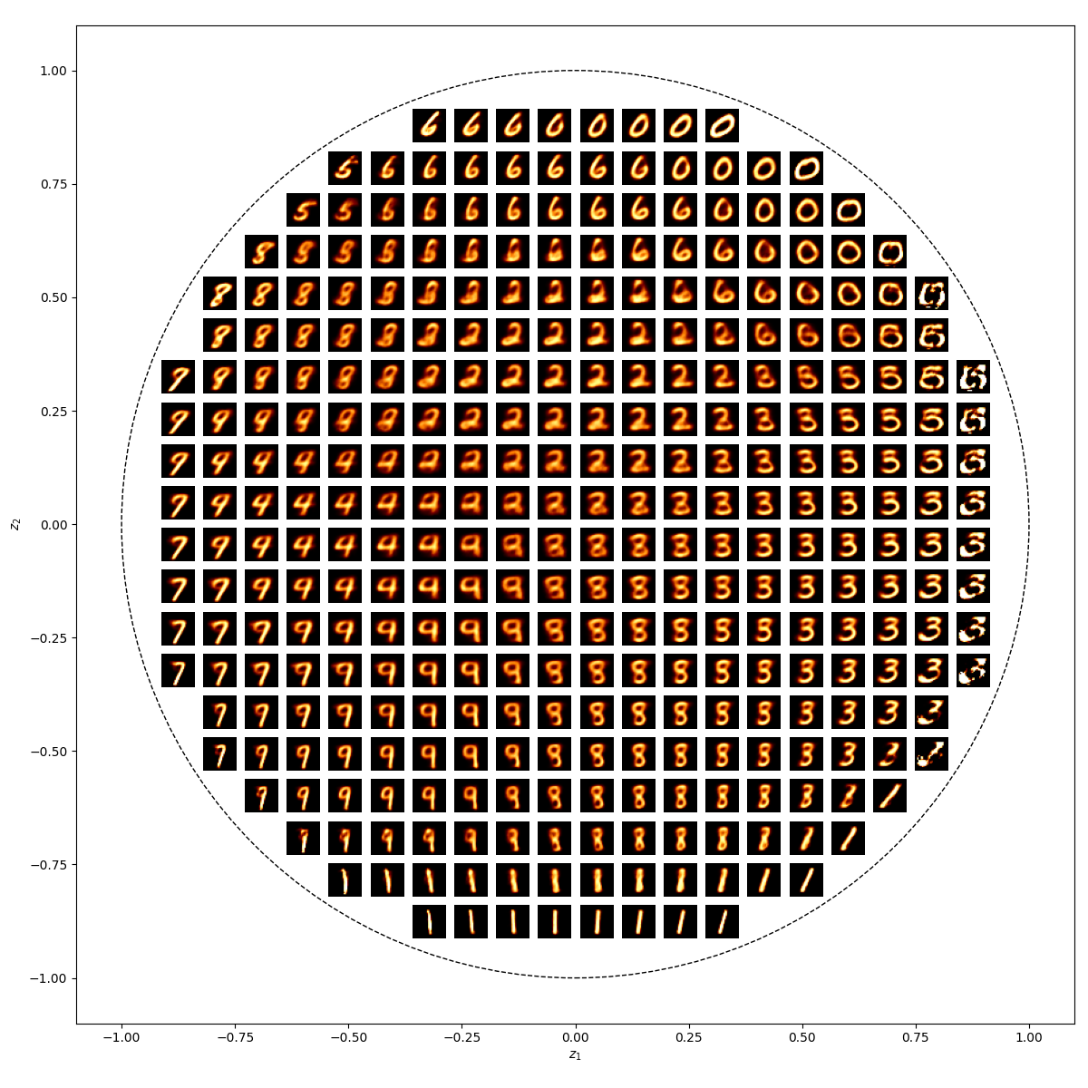
So if the issue is that they all pulled towards some central region for regularisation through the normal prior centred at 0, what if we eliminate the ‘centre’ but retain the probabilistic interpretation so we get the best of both worlds, and define the distribution on a sphere. The samples live on this sphere, and so in this space there is no ‘centre’3. This idea motivates the concept of hyperspherical VAEs.

This looks much better! (separation wise)
So we can try to learn a conditional distribution on the latent parameters on the sphere which mitigates the pull of the ‘centre’ but still regularise the space using distributions defined on the sphere. The next few sections will be dedicated to exploring this idea.
It might seem like a bit of an abstraction, and cards on the table oh boi it is, but you likely already think somewhat in terms of non-euclidean spaces already. e.g.
- To a very close approximation, you exist on a sphere (although idk, if I have any readers that are astronauts hit me up). You technically reside in 3D space however, if a person is flying a plane a very long distance (say Melbourne to Sapporo) you won’t tell them the downwards coordinate to go straight through the Earth! (we are thinking in terms of spherical spaces here)
- You can imagine navigating social media as some weird object. Everyone is friends or follows Obama, so you can think that Obama is close to everyone. But just because two people follow Obama, doesn’t mean that they are friends or follow each other at all (this is a behaviour that is common in hyperbolic spaces).

And it turns out that some data is better represented in these spaces e.g. as shown in Bronstein et al. 2017.
Hyperspherical VAE
von Mises-Fisher Distribution
The von Mises-Fisher distribution is essentially the replacement distribution in the VAE instead of a traditional normal distribution. It is described as the normal distribution on a sphere and has the following PDF,
\[\begin{align} f_{vMF}(\vec{x} | \vec{\mu}, \kappa) = \frac{\kappa^{p/2-1}}{(2\pi)^{p/2}I_{p/2-1}(\kappa)} \exp(\kappa \vec{\mu}^T\vec{x}). \end{align}\]This to me, makes no sense on the face of things.
von Mises Distribution
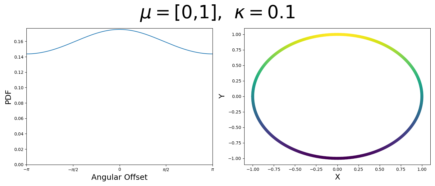
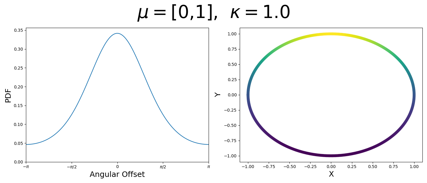
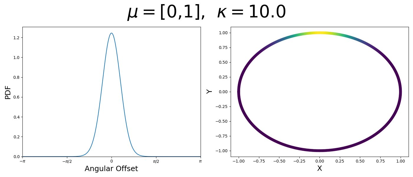
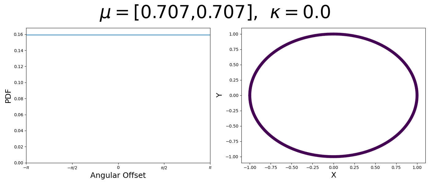
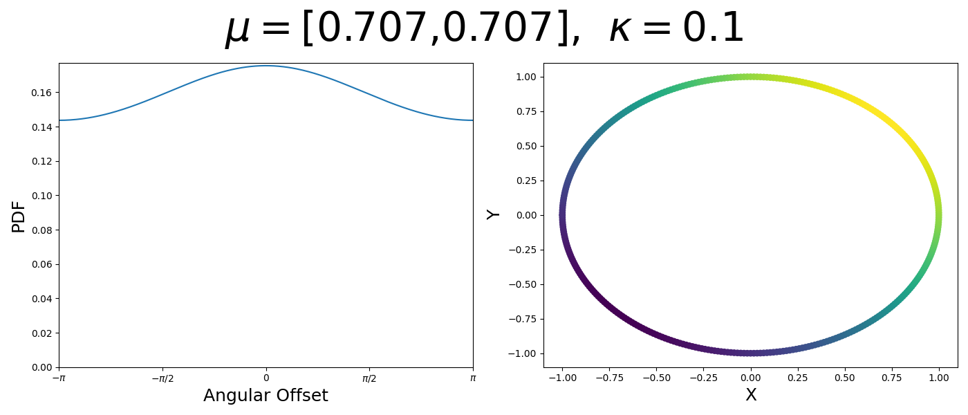
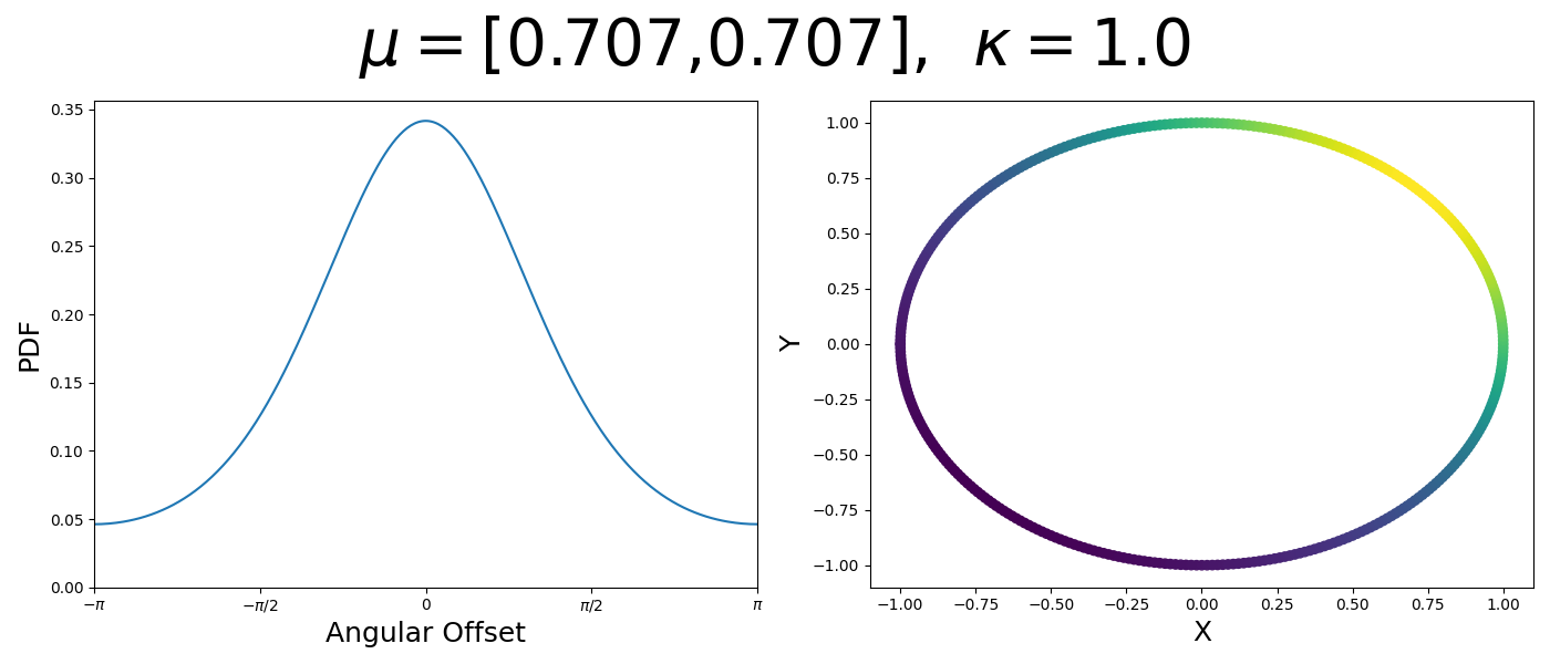
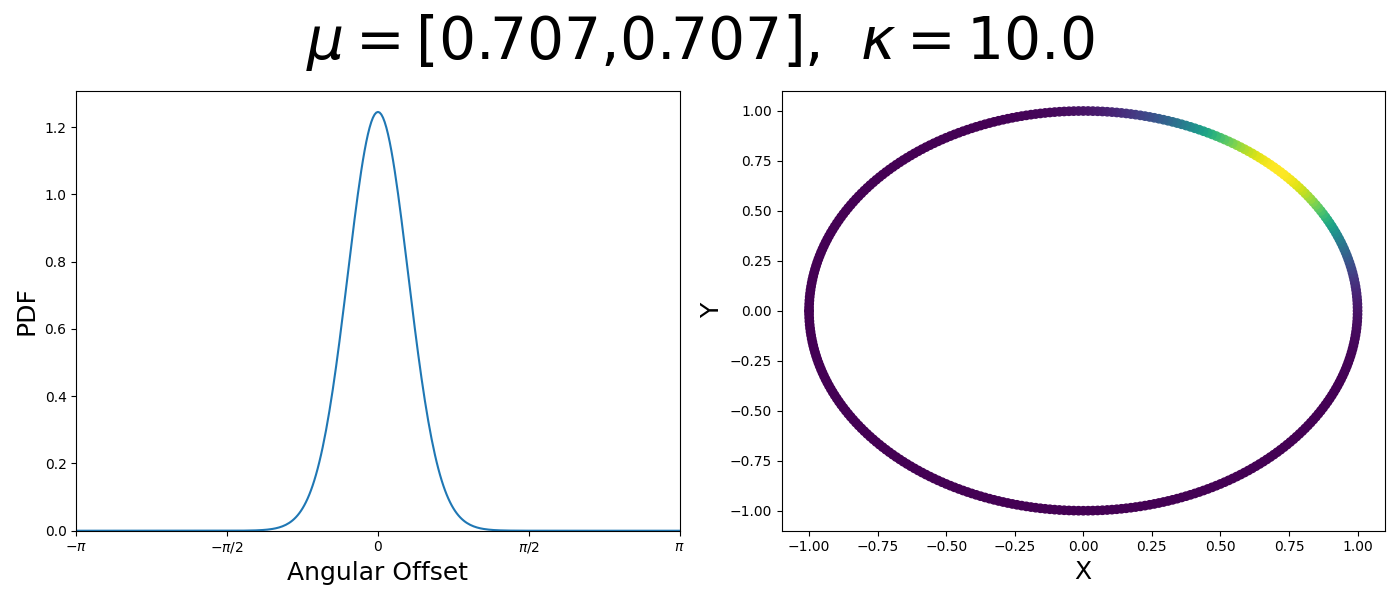
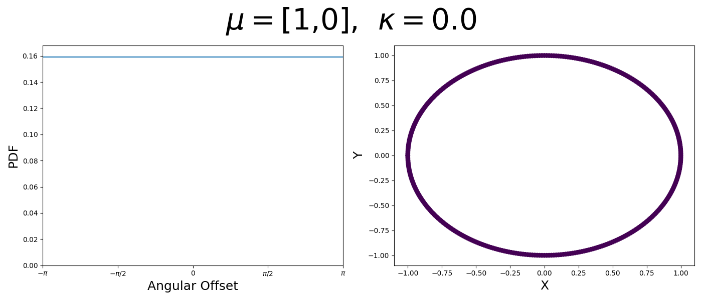
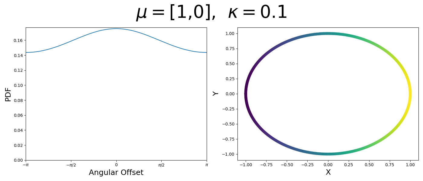
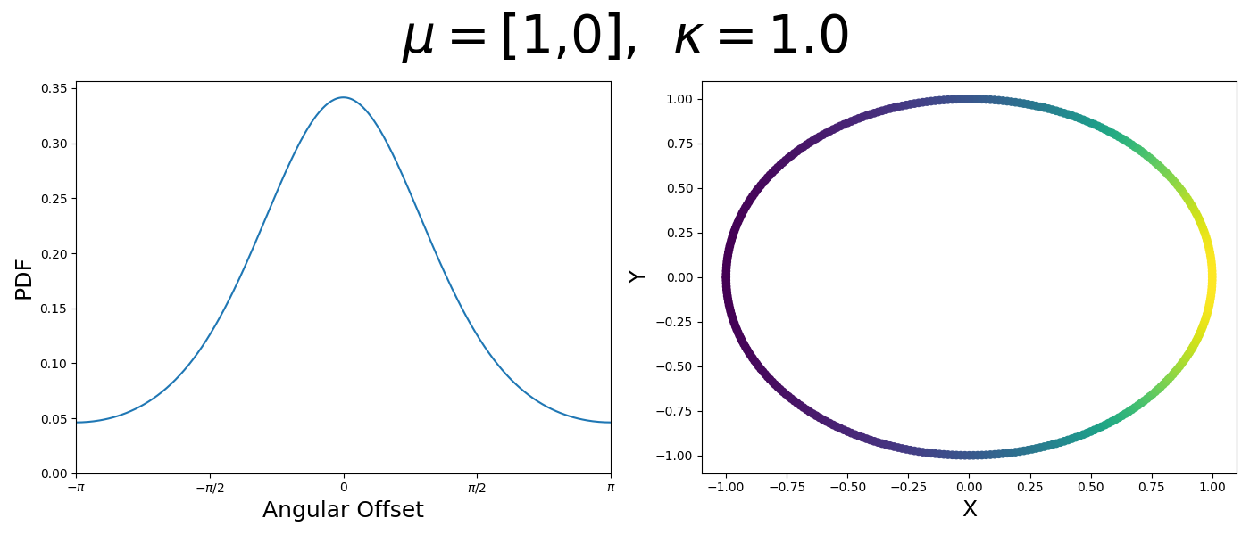
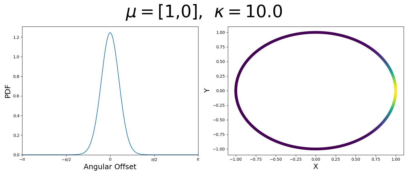
So let’s first look at the simpler case where \(p=2\), i.e. the circle, called the von-Mises distribution. It has the following PDF,
\[\begin{align} f_{vM}(\vec{x} | \vec{\mu}, \kappa) = C(\kappa) \exp(\kappa \vec{\mu}^T\vec{x}). \end{align}\]Where \(C(\kappa)\) will just be a normalisation factor to us for now. In the case where \(\vec{\mu}\) and \(\vec{x}\) have unit length (which we will presume they do as they exist on the unit circle), then the dot product inside the exponential simplifies to the cosine of the angle between the two vectors, \(\theta_{x\mu}\).
\[\begin{align} f_{vM}(\vec{x} | \vec{\mu}, \kappa) = C(\kappa) \exp(\kappa \cos(\theta_{x\mu})). \end{align}\]So \(\cos(\theta_{x\mu})\) will take a maximal value of 1 when the two vectors are parallel and minimal value of -1 when they are anti-parallel. Because \(\vert \cos(\theta_{x\mu})\vert \leq 1\) then the exponent will always be less than or equal to 1 as well. So the absolute difference in angle is similar to how the normal distribution is only dependent on the absolute difference between two values, with \(\kappa\) acting much like the variance in a traditional normal distribution.
It also turns out that the normalisation factor has a bessel function in it, but for now we don’t need to worry about that.
\[\begin{align} C(\kappa) = \int_{-\pi}^{\pi} \exp(\kappa \cos(x)) dx = 2\pi I_0(\kappa), \end{align}\]where \(I_0(\kappa)\) is the modified Bessel function of the first kind of order 0.
Let’s have a look at this distribution as a function of angle as well as on the actual circle.

Back to the von Mises-Fisher Distribution
So back to the full distribution, I’ll actually explain it in detail now.
\[\begin{align} f_{vMF}(\vec{x} | \vec{\mu}, \kappa) = \frac{\kappa^{p/2-1}}{(2\pi)^{p/2}I_{p/2-1}(\kappa)} \exp(\kappa \vec{\mu}^T\vec{x}). \end{align}\]The \(p\) denotes the dimension of the sphere +1. So for a sphere in 3D ambient space then \(p=3\).
Once again, let’s have a look at what the distribution implies for different parameters, particularly \(p=3\) and \(\mu=[1, 0, 0]\). (i.e. we’ll be looking at how the spread parameter \(\kappa\) works)

So broadly the von Mises-Fisher distribution boils down to,
\[\begin{align} f_{vMF}(\vec{x}\vert\vec{\mu}, \kappa) \propto \kappa^{p/2 - 1} \exp(\kappa \vec{\mu} \cdot \vec{x}), \end{align}\]where again we can make the comparisons to the traditional normal distribution. \(\kappa\) works similar to inverse variance, and instead of asking how similar a vector is to the mean by finding the absolute norm squared \(\lVert \vec{x} - \vec{\mu}\rVert^2\), we quantify the similarity through the cosine similarity or simply the dot product \(\vec{\mu} \cdot \vec{x}\) when the two vectors have unit magnitude. We just get something weird in the normalisation constant because of the form of our distribution.
Reparameterisation Trick with the von Mises-Fisher distribution
This is all great, well and good now instead of learning a mean vector and standard deviation vector as intermediates in our VAEs latent distributions, we can learn the mean direction vector and \(\kappa\)! However, standard VAEs rely quite heavily on the reparameterisation trick which allows us to “inject” the stochasticity of sampling into the training procedure.
i.e. We create some noise through the variable \(\vec{\epsilon}\) that we say comes from a standard normal with the same dimensionality as our latent space, \(\vec{\epsilon} \sim \mathcal{N}(\vec{0}, \vec{1})\) then we could sample the conditional gaussian in this space by \(z = \vec{\sigma} \odot \vec{\epsilon} + \vec{\mu}\).
This meant when we were optimising/taking derivatives with respect to \(\vec{\sigma}\) and \(\vec{\mu}\) we would get pretty simple answers, either \(\vec{\epsilon}\) or \(\vec{1}\). Or in more mathematically rigorous way, our loss can be represented on some level as an expectation of some function.
\[\begin{align} L(\vec{\mu}, \vec{\sigma}, \vec{\phi}) = \mathbb{E}_{\vec{z} \sim q(\vec{z}|\kappa, \vec{\mu})}\left[f_\vec{\phi}(z) \right], \end{align}\]when optimising we then need to taking derivatives with respect to the parameters we are optimising… which are within the expectation which is hard or at least the estimator, called the REINFORCE estimator you get out has quite high variance. But if we can perform the reparameterisation trick then we can pull the derivative inside the expectation. For example with respect to \(\vec{\mu}\) we can calculate the derivatives as,
\[\begin{align} \nabla_{\vec{\mu}} L(\vec{\mu}, \vec{\sigma}, \vec{\phi}) &= \nabla_{\vec{\mu}} \left( \mathbb{E}_{\vec{\epsilon} \sim \mathcal{N}(\vec{0}, \vec{1})}\left[f_\vec{\phi}(z = \vec{\mu} + \vec{\sigma} \odot \vec{\epsilon}) \right]\right) \\ &= \mathbb{E}_{\vec{\epsilon} \sim \mathcal{N}(\vec{0}, \vec{1})}\left[ \nabla_{\vec{\mu}} f_\vec{\phi}(z = \vec{\mu} + \vec{\sigma} \odot \vec{\epsilon}) \right] \end{align}\]But how do we do this for the von Mises-Fisher distribution…? We can’t use the same trick, sampling \(\vec{\epsilon}\) uniformly on the sphere for example, as we don’t (currently) have a way to taking a mean vector and \(\kappa\) and stay on the sphere. So what do we do??
One of the main results of the paper Hyperspherical Variational Auto-Encoders by Davidson et al. (2018) was basically this trick for the hypersphere.
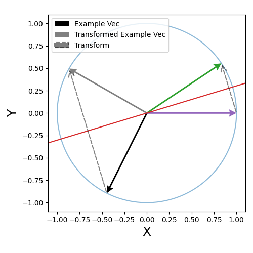
It basically comes down to using the symmetry of the vMF (von Mises-Fisher) distribution. If you just rotate the sphere (/change your perspective) you can always make it so that the samples around the mean vector are centred around the vector in the first dimension \(\vec{e}_1 = [1,0,0,...,0]\). We can then sample some 1D rejection sampling distribution about this direction to encode the spread.
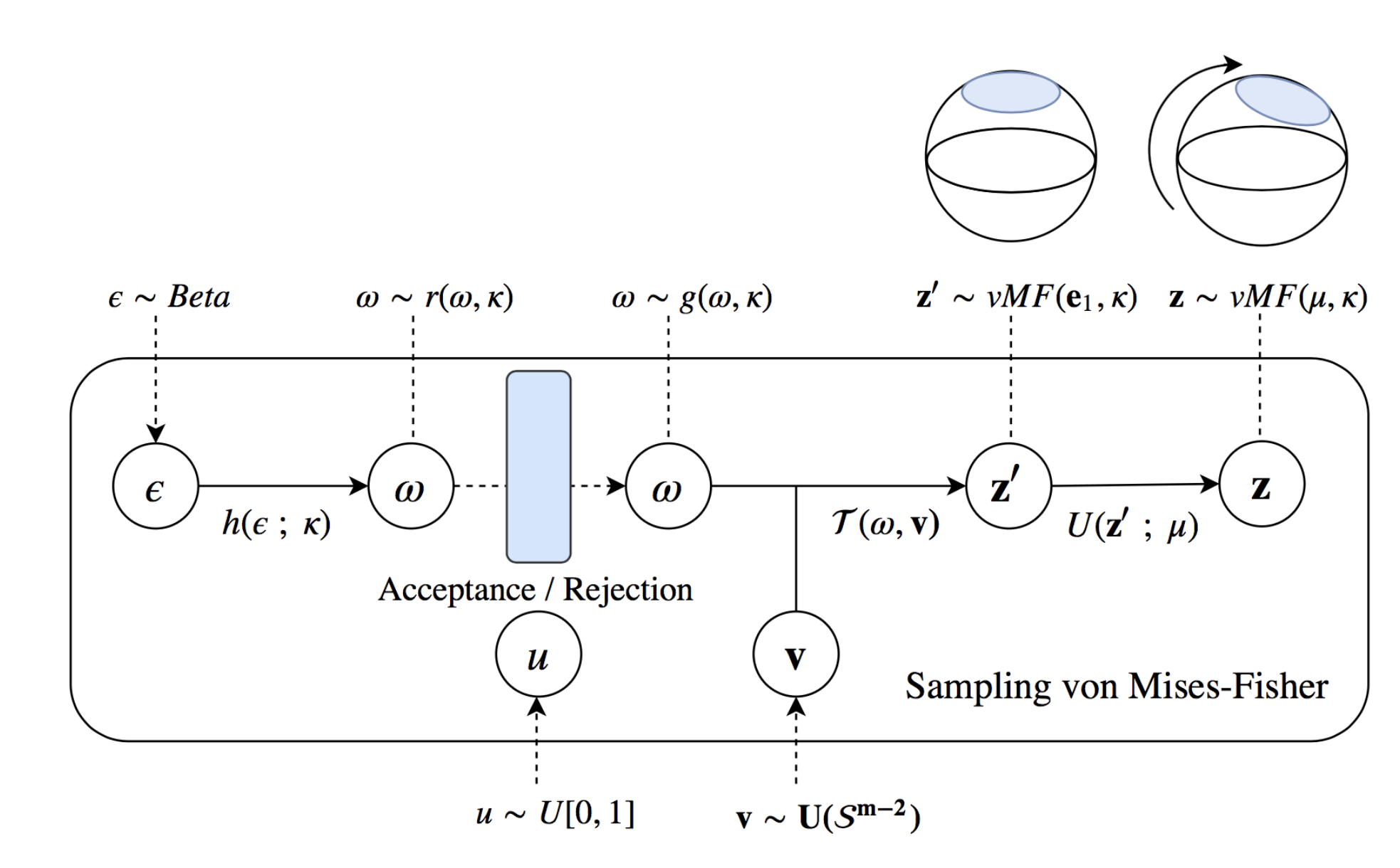
The basic idea of the sampling is shown in the below figure which I took from Davidson et al. (2018), which shouldn’t make complete sense yet.
If you’re alright with the picture so far, that we have a spherical distribution, and we have some method to do something similar to the reparameterisation trick with this distribution, you can move on to the next section. For the rest of this section we’ll try and learn how this trick actually works.
The deets
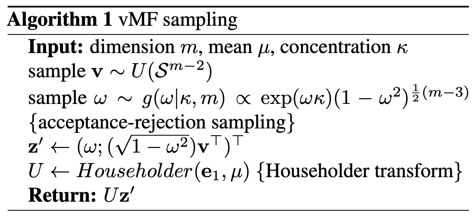
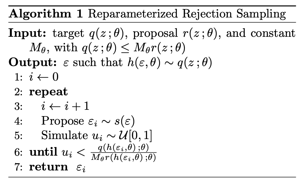
To sample the vMF distribution with something like the reparameterisation trick, there are only four steps (plain english version of Algorithm 1 from Davidson et al. (2018)).
- Generate samples on the unit sphere 1-dimension less than the dimension you want (we’ll refer to this as \(\vec{v} \sim U(\mathcal{S}^{m-2})\))
- Sample the spread due to \(\kappa\) (where we sample the equivalent \(\vec{\epsilon}\)) in the first dimension from some weird distribution \(g(\omega, \kappa)\)
- Scale the previously uniform samples to add the first dimension of samples. Now getting samples on the full sphere \(z' = (\omega;(\sqrt{1-\omega^2})\vec{v}^T)^T\)
- Rotate the distribution so that the samples are centred around the mean vector \(\vec{\mu}\) (using the Householder transform)
This is encapsulated in the below function sample_vMF.
from scipy.stats import uniform_direction
import numpy as np


def sample_vMF(mean_vec, k, num=10):

    m = len(mean_vec)

    e1vec = np.zeros(m)
    e1vec[0] = 1.

    # Step 1
    uniform_sphere_samples = uniform_direction(dim=m-1).rvs(num)
    #-----

    # Step 2
    W = sample_vMF_mixture(k, m, num=num)
    #-----

    # Step 3
    adjusted_u_sphere_samples = (np.sqrt(1-W**2) * uniform_sphere_samples.T).T
    zprime = np.concatenate((W[:, None], adjusted_u_sphere_samples), axis=1)
    #-----

    # Step 4
    U = householder(mean_vec, e1vec)
    z = (zprime @ U)
    #-----

    return z
The first step, getting \(\vec{v}\sim U(\mathcal{S}^{m-2})\), is pretty easy actually. You can sample any rotationally symmetric distribution and scale the samples to be on the unit sphere. e.g. The multivariate normal distribution with 0 mean and covariance. For us we’ll just use the scipy.stats.uniform_direction distribution for simplicity.
The second step was by far the hardest to wrap my head around, so I’ll cover the other two first.
Presuming that you have samples about the first dimension that represent the spread from \(\kappa\), we need to modify the other uniform samples on the sphere such that together, everything is still on the sphere. By some simple algebra you can see that
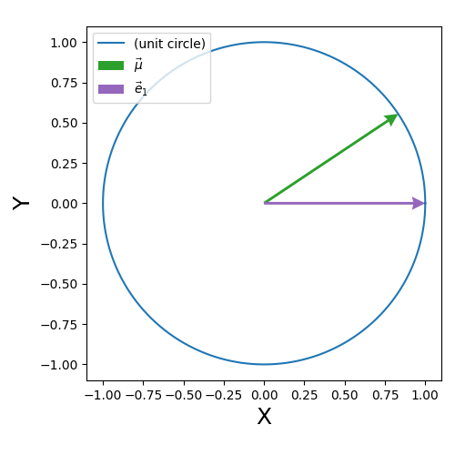
\[\begin{align} z' \cdot z' &= \omega^2 + (1-\omega^2) \vec{v} \cdot \vec{v} \\ &= \omega^2 + (1-\omega^2) \\ &= 1 \text{ }. \end{align}\]The final step that constructs \(U\) that transforms our samples about \(\vec{e}_1\) to \(\vec{\mu}\) is done by the householder transform or reflection. Essentially creates a plane between the direction vector \(\vec{\mu}\) and \(\vec{e}_1\) such that if you reflect about it, \(\vec{e}_1\) turns into \(\vec{\mu}\). The actual transform is given as,
\[\begin{align} U = I - \hat{u} \, \hat{u}^T, \end{align}\]where \(\hat{u}\) is the unit vector in the direction of \(\vec{e}_1 - \vec{\mu}\).
There’s a tonne of useful videos and lectures notes on this that I’d recommend for a more rigorous take on this operation (this YouTube video seemed pretty good but I’d put them on 2x speed) but I include a little diagram for some quick visual intuition below.


The operation is encoded in the householder function below (pretty much the same as Algorithm 3 from Davidson et al. (2018)).
def householder(dirvec, e1vec):

    uprime = e1vec - dirvec

    uprime /= np.linalg.norm(uprime)

    U = np.eye(len(e1vec)) - 2*uprime[:, None]*uprime[None, :]

    return U
Sampling the mixture distribution
Now let’s circle back to the second step. For this we need to motivate two things:
- Splitting the distribution such that the we can sample the 1D mixture distribution \(g(\omega\vert \kappa, m)\) and
- basically how to efficiently sample this function in a ‘reparameterisation trick’-y way.
1. Splitting the distribution
Splitting the distribution into two is actually fairly intuitive when observing the problem from a specific frame.
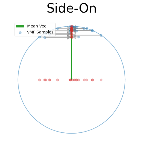
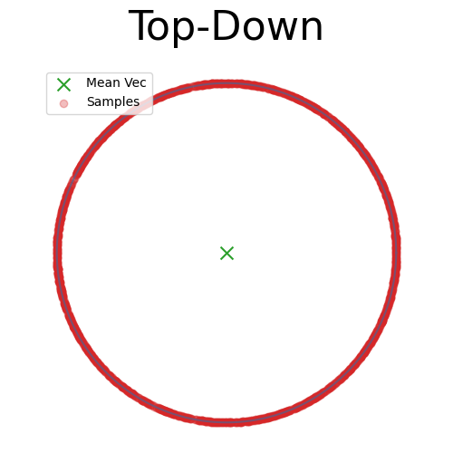
I’ll try and walk through this with a 3D example. We have the mean vector and the sphere.
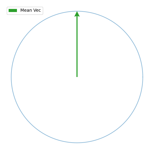
Let’s just presume that we can generate some samples for now.
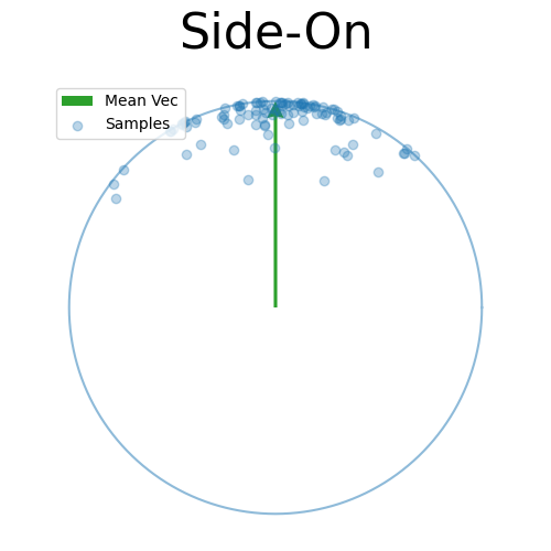
What we’re really looking at here is a 3D plot but that’s hard to get right in matplotlib due to it’s bad ordering behaviours.
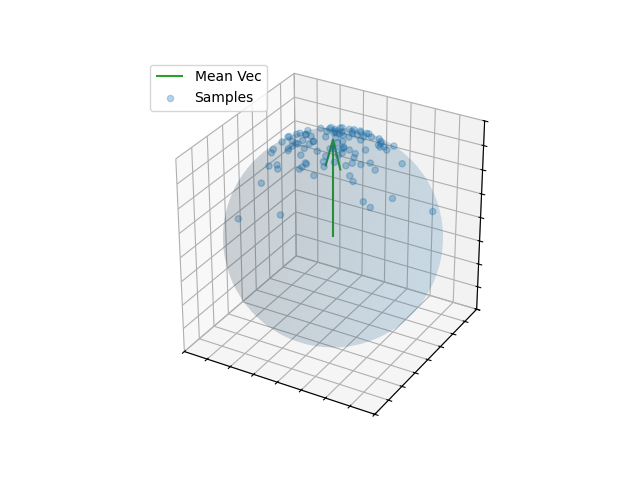
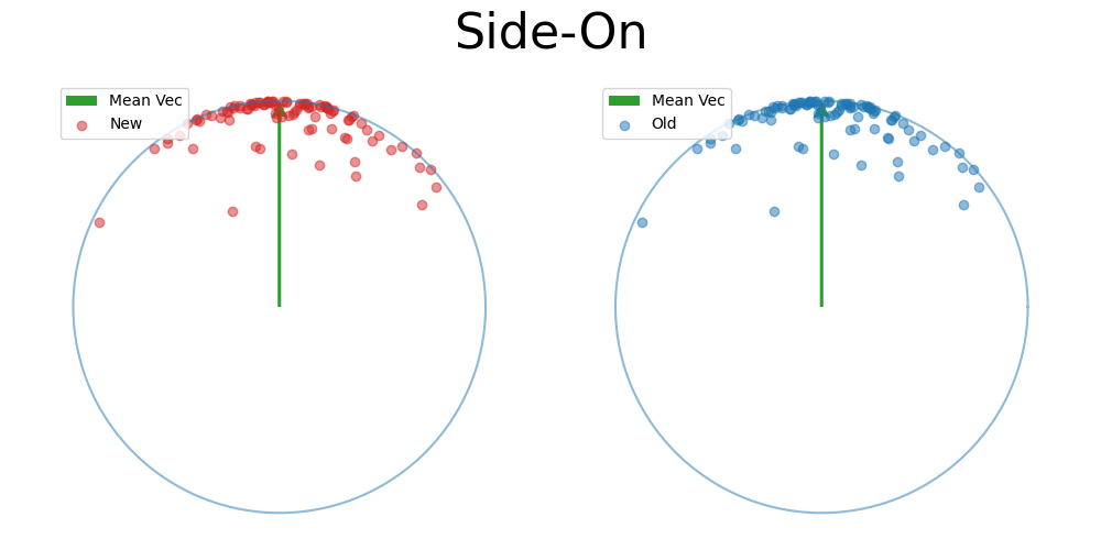
Back to the 2D side-on view, because the samples are symmetric about the mean vector we can kind of see that the spread due to \(\kappa\) can be mostly attributed along this direction, and then the samples in the other directions are uniform in direction.
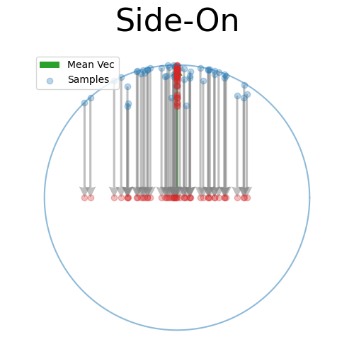
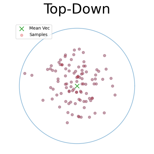
Again, just presuming that this will work for now, let’s scale the samples in the other dimensions such that they fall on the sphere 1-dimension lower than our original one (in this case the circle).
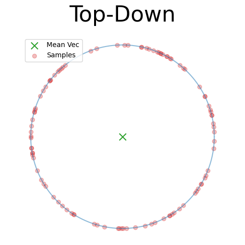
Adding a few more samples we can then look at the angular distribution confirming that it’s uniform on the sphere because it’s uniform in angle.
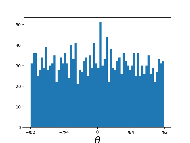
Going back to the lower number of samples,
we can then pretend that we sampled the first dimension via some complicated distribution accounting for the spread (getting \(\omega\)), and scale our uniform samples on \(\vec{v} \sim S^{1}\) back to \(S^{2}\) via \((\omega, \sqrt{1-\omega^2} \vec{v}^T)\) (but in reality just take the projected values from the beginning) to see that we recover the exact same distribution.
So this really implies that we can uniformly sample the sphere 1-dimension lower than the one we want, sample some 1D distribution, and then scale our samples with the 1D variable as a new dimension as a way to sample the vMF.
If you want a more rigorous explanation, then I’m going to have to refer to the same papers that Davidson et al. (2018) refer to called “Computer Generation of Distributions on the M-sphere” (1984) by Gary Ulrich and the paper that Ulrich cites called “A Family of Distributions on the m-Sphere and Some Hypothesis Tests” (1978) by John G. Saw.
2. Sampling the 1D Mixture distribution in a ‘reparameterisation trick’-y way
So hopefully we now understand why we can split the distribution in two where \(\vec{z} = (\omega, (\sqrt{1-\omega^2})v^T)\) with \(f(\vec{z}\vert\kappa, m) = g(\omega \vert \kappa, m) \cdot g_2(\vec{v} \vert m-1)\). We can sample \(\vec{v}\) by scaling samples from the multivariate standard normal distribution (as the samples are directionally uniform/symmetric). But what is \(g(\omega \vert \kappa, m)\), and how do we sample it in a ‘reparameterisation trick’-y way?
The general method will be:
- We take samples from a distribution that we can already sample efficiently that has a similarish form to \(g(\omega \vert \kappa, m)\)
- We perform rejection sampling with these samples, where the probability of accepting the values is the ratio of \(g(\omega \vert \kappa, m)\) and our proposal distribution
- Figure out how this gives us derivatives of the loss that doesn’t involve a derivative of the distribution over which we are taking an average
To save some time (for both you and me) we’re just going to propose that,
\[\begin{align} g(\omega \vert \kappa, m) &\propto \exp(\kappa \vec{e}_1 \cdot x) (1-\omega^2)^{(m-3)/2} \\ &=\exp(\kappa \omega) (1-\omega^2)^{(m-3)/2}, \end{align}\]which in essence is the von Mises-Fisher distribution with a geometrical jacobian factor for what would be a surface integral. Accounting for the surface area of lower dimensional sphere with the dimensions perpendicular to \(\vec{e}_1\) ((where we get the uniform samples) ), \(\text{Area} \propto R^{m-2} = (1-\omega^2)^{\frac{m-2}{2}}\), and the conversion between \(\omega\) as a z-coordinate and \(\phi\) in angular coordinates (as any integration has to be done on the sphere),
\[\begin{align} d\omega &= d(\cos(\phi)) = -\sin(\phi) d\phi \\ d\phi &= d\omega/\sqrt{1-\cos^2(\phi)} = d\omega/\sqrt{1-\omega^2}\\ \implies J(\omega) &= (1/\sqrt{1-\omega^2}) \cdot (1-\omega^2)^{\frac{m-2}{2}} \\ J(\omega) &= (1-\omega^2)^{\frac{m-3}{2}}. \\ \end{align}\]So that gives us the form of \(g(\omega \vert \kappa, m)\) (up to some multiplicative constant with respect to \(\omega\)). Next, we are going to guess that we can sample our noise from the following distribution (this similar to the bit in the reparameterisation trick where we sample from a distribution independent of our parameters to get the stochastic component),
\[\begin{align} \epsilon \sim s(\epsilon) = \text{Beta}(\frac{m-1}{2}, \frac{m-1}{2}), \end{align}\]and then transform it to make a proposal for \(\omega\) as,
\[\begin{align} \omega = h(\epsilon \vert \kappa, m) = \frac{1-(1+b(\kappa, m))\epsilon}{1-(1-b(\kappa, m))\epsilon}, \end{align}\]we’ll get to the specific form of \(b\) later, for now you can just imagine that it’s some simple combination of \(\kappa\) and \(m\).
The \(r(\omega, \kappa)\) referred to in the paper is the so called envelope distribution used in rejection sampling. For a thorough introduction to rejection sampling I would recommend my blog post (not biased at all…).
The basics of it is that the envelope is some other distribution that we can sample, and then after some multiplicative factor, we reject samples with a smaller probability than the actual distribution. Differences between good and bad envelopes is exemplified in the below two GIFs. One has a non-informative envelope (top one with a uniform distribution) and one has an infomative envelope (bottom, gaussian envelope). You can observe that one wastes more proposals (orange dots) than the other.


What we want, is the envelope to have as similar of a form as the distribution we are trying to sample from. If we look at the implied distribution on \(\omega\), based on injecting the samples/density in \(s(\epsilon)\) into \(h(\epsilon \vert \kappa, m)\) we find that we’ve actually already done this. First we need to rearrange \(\epsilon\) in terms of \(\omega\), i.e. \(\epsilon = h^{-1}(\omega\vert\kappa, m)\).
\[\begin{align} \omega &= \frac{1-(1+b)\epsilon}{1-(1-b)\epsilon} \\ \left(1-(1-b)\epsilon\right)\omega &= 1-(1+b)\epsilon \\ \omega-\omega(1-b)\epsilon &= 1-(1+b)\epsilon \\ \omega - 1 &= (\omega(1-b)-(1+b))\epsilon \\ \epsilon &= \frac{\omega - 1}{\omega(1-b)-(1+b)} \\ \end{align}\]This allows us to get the jacobian between \(\epsilon\) and \(\omega\) in terms of \(\omega\).
\[\begin{align} \frac{d\epsilon}{d\omega} &= \frac{-2b}{(1+b - \omega(1-b))^2}. \\ \end{align}\]Hence,
\[\begin{align} r(\omega\vert\kappa, m) &= \left\lVert\frac{d\epsilon}{d\omega}\right\rVert s(\epsilon(\omega)) \\ &= \left\lVert\frac{d\epsilon}{d\omega}\right\rVert \epsilon^{\frac{m-3}{2}}\left(1-\epsilon\right)^{\frac{m-3}{2}} \\ &= \frac{2b}{(1+b - \omega(1-b))^2} \left(\frac{\omega - 1}{\omega(1-b)-(1+b)}\right)^{\frac{m-3}{2}}\left(1 - \frac{\omega - 1}{\omega(1-b)-(1+b)}\right)^{\frac{m-3}{2}} \\ &= \frac{2b}{(1+b - \omega(1-b))^2} \left(\frac{\omega - 1}{\omega(1-b)-(1+b)}\right)^{\frac{m-3}{2}}\left(\frac{\omega(1-b)-(1+b) - \omega + 1}{\omega(1-b)-(1+b)}\right)^{\frac{m-3}{2}} \\ &= \frac{2b}{(1+b - \omega(1-b))^2} \left(\frac{\omega - 1}{\omega(1-b)-(1+b)}\right)^{\frac{m-3}{2}}\left(\frac{\omega -b\omega - 1 - b - \omega + 1}{\omega(1-b)-(1+b)}\right)^{\frac{m-3}{2}} \\ &= \frac{2b}{(1+b - \omega(1-b))^2} \left(\frac{\omega - 1}{\omega(1-b)-(1+b)}\right)^{\frac{m-3}{2}}\left(\frac{-b( \omega + 1)}{\omega(1-b)-(1+b)}\right)^{\frac{m-3}{2}} \\ &= \frac{2b^{\frac{m-1}{2}}}{(1+b - \omega(1-b))^2} \left(\frac{(1 - \omega)(1 + \omega)}{(\omega(1-b)-(1+b))^2}\right)^{\frac{m-3}{2}} \\ &= 2b^{\frac{m-1}{2}} \frac{(1 - \omega^2)^{\frac{m-3}{2}} }{(1 + b - \omega(1-b))^{m-1}}\\ \end{align}\]The key similar here, and again we want the envelope to be as similar to the distribution we are trying to sample, is that they both share a \((1 - \omega^2)^{\frac{m-3}{2}}\) factor. The polynomial factor actually roughly gets larger with larger \(\omega\), which is also similar to \(\exp(\kappa \omega)\), but crucially will always be larger than \(\exp(\kappa \omega)\) within the range of \(\omega\). i.e. We’ve found a pretty good envelope.
The actual sampling then comes down to rejection sampling using \(s(\epsilon)\), \(r(\omega\vert\kappa, m)\) (dependence on \(\kappa\) comes through \(b\) by the way) and \(g(\omega\vert\kappa, m)\). This process is described in Algorithm 2 from Davidson et al. (2018) with some algebraic trickery that I’m not going to go into as to me at least, that’s all it is.
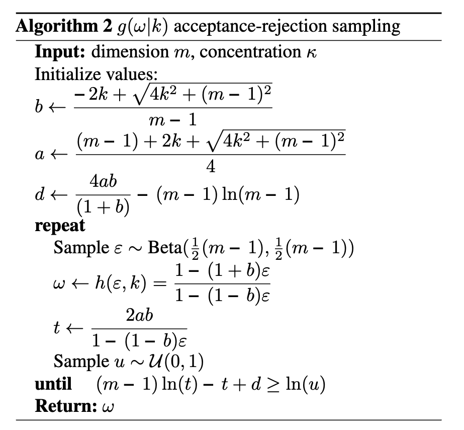
I’ve coded this up in the below python function.
from scipy.stats import beta, uniform, uniform_direction

def sample_vMF_mixture(k, m, num=10):
    b = (-2*k + np.sqrt(4*k**2 + (m-1)**2))/(m-1)
    a = ((m-1) + 2*k + np.sqrt(4*k**2 + (m-1)**2))/4
    d = 4*a*b/(1+b) - (m-1)*np.log(m-1)


    samples = []

    condition = True
    while condition:
        Y = beta((m-1)/2, (m-1)/2).rvs()
        u = uniform(0, 1).rvs()
        W = (1 - (1 + b) * Y)/(1 - (1 - b) * Y)

        T = 2*a*b/(1 - (1-b)*Y)

        if (m-1)*np.log(T) - T + d > np.log(u):
            samples.append(W)

            if len(samples)==num:
                condition = False
    return np.array(samples)
Putting it all together
We can then put this into action with the function we defined way above.
custom_vMF_samples = sample_vMF(np.array([0., 0., 1.0]), 5.0, num=5000)
Voila! Terrifique! Magnifique! (Not sure if that’s how I’m meant to spell that!)
Taking Derivatives
So we made a sampling regime similar to the standard reparameterisation trick, but the key thing in the original was that the derivatives of the loss worked out. The next question we need to ask ourselves is whether that is the case?
It’s not immediately obvious because what we did isn’t an exact 1-to-1 to the original, because of the rejection sampling step (which isn’t in the original).
What Davidson et al. (2018) do is use a result from “Reparameterization Gradients through Acceptance-Rejection Sampling Algorithms” - Naesseth et al. (2016). In this paper they show that for many rejection sampling setups you can move gradients of the parameters being optimised, into the expectations within the loss.
If we represent our loss as some expectation over the KL divergence between some exact posterior probability distribution \(p(z\vert x) = p(x, z)/p(x)\) and our (variational) approximation \(q(z\vert x ; \phi)\) that we are optimising with respect to \(\phi\) (for those familiar with variational inference I’m just quickly deriving the ELBO),
\[\begin{align} KL(q\vert\vert p ; \phi) &= \mathbb{E}_{z\sim q(z\vert x)}\left[ \log \frac{q(z\vert x ; \phi)}{p(z\vert x)}\right] \\ &= \mathbb{E}_{z\sim q(z\vert x)}\left[ \log q(z\vert x ; \phi) - \log p(z\vert x) \right] \\ &= \mathbb{E}_{z\sim q(z\vert x)}\left[ \log q(z\vert x ; \phi) - \log p(z, x) + \log p(x) \right] \;\;\;\;\;\;\ \text{(Bayes' theorem)}\\ &= \mathbb{E}_{z\sim q(z\vert x)}\left[ \log q(z\vert x ; \phi)\right] \\ &\;\;\;\;- \mathbb{E}_{z\sim q(z\vert x ; \phi)}\left[\log p(z, x)\right] \\ &\;\;\;\;+ 1 \cdot \log p(x). \;\;\;\;\;\;\ \text{(p(x) doesn't involve z)}\\ \end{align}\]If we are constructing a loss to optimise, then that last term doesn’t matter as it doesn’t involve \(\phi\) so we will drop it. Also in statistics the first term has a more formal definition as the entropy of \(q(z\vert x ; \phi)\), denoted \(\mathbb{H}[q(z\vert x ;\phi)]\). We will then follow the notation of Naesseth et al. (2016) and denote the remaining term as the following (dropping the dependence on \(x\) from now on, presuming it to be a constant effectively),
\[\begin{align} \mathbb{E}_{z\sim q(z; \phi)}\left[\log p(z, x)\right] = \mathbb{E}_{z\sim q(z; \phi)}\left[f(z)\right]. \end{align}\]We will then write the loss, or simply the function that we are trying to minise, as,
\[\begin{align} L(\phi) = \mathbb{E}_{z\sim q(z ; \phi)}\left[f(z)\right] + \mathbb{H}[q(z ;\phi)]. \end{align}\]What Naesseth et al. (2016) then show is that if you have a target distribution that you are trying to sample, in this case \(q(z;\phi)\), a proposal distribution \(r(z;\phi)\) and constant \(M_\phi\) such that \(q(z;\phi)\leq M_\phi r(z;\phi)\). We perform rejection sampling following the algorithm below that I’m stealing from Naesseth et al. (2016) because I cannot figure out how to do the formatting for algorithms in GitHub markdown (just replace the \(\theta\)’s with \(\phi\)’s).
When the sampling is set up in this manner we can represent the probability of accepting a given sample as the folliwing (following very closely to equation 4 in Naesseth et al. (2016)),
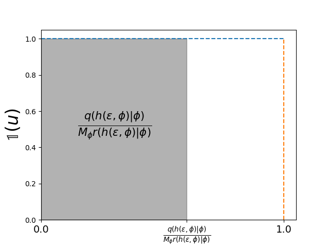
\[\begin{align} \pi(\epsilon;\phi) = \int \pi(\epsilon, u ;\phi) du \end{align}\]\(\pi(\epsilon, u ;\phi)\) is the probability of accepting a given \(\epsilon\) for a specific \(u\). We can split this into the base probability of sampling a given \(\epsilon \sim s(\epsilon)\) and indicator function (denoted \(\mathbb{1}\)) for whether we accept this given \(\epsilon\), along a normalisation constant which turns out to be \(M_\phi\).
\[\begin{align} \pi(\epsilon;\phi) &= \int \pi(\epsilon, u ;\phi) du \\ &= \int M_\phi s(\epsilon) \mathbb{1} \left[0 < u < \frac{q(h(\epsilon, \phi) ; \phi)}{M_\phi r(h(\epsilon, \phi) ; \phi)} \right] du \\ &=M_\phi s(\epsilon) \int \mathbb{1} \left[0 < u < \frac{q(h(\epsilon, \phi) ; \phi)}{M_\phi r(h(\epsilon, \phi) ; \phi)} \right] du \\ \end{align}\]Where \(h(\epsilon, \phi)\) still represents the transform between \(\epsilon\) and the parameter of interest \(z\) which for our specific use-case is \(\omega\). The integration then follows that,
\[\begin{align} \pi(\epsilon;\phi) &=M_\phi s(\epsilon) \int \mathbb{1} \left[0 < u < \frac{q(h(\epsilon, \phi) \vert \phi)}{M_\phi r(h(\epsilon, \phi) ; \phi)} \right] du \\ &= s(\epsilon) \frac{q(h(\epsilon, \phi) ; \phi)}{r(h(\epsilon, \phi) ; \phi)},\\ \end{align}\]which if doesn’t make sense I’ve attempted to represent the indicator function graphically below. The function outputs 1 until it hits the threshold so the integral of it with respect to \(u\) just ends up being the threshold.
And once we have the above form of \(\pi\) we can re-write our loss as the following,
\[\begin{align} L(\phi) &=\mathbb{E}_{\epsilon \sim \pi(\epsilon ; \phi)}\left[f(h(\epsilon, \phi))\right] + \mathbb{H}_{\epsilon \sim \pi(\epsilon ; \phi)}[q(h(\epsilon, \phi) ;\phi)]. \end{align}\]Now that we have the rejection sampling distribution encoded like this it’s pretty simple to take derivatives of our loss. Like Naesseth et al. (2016) I’ll focus on the first term, as the derivation for the second is basically exactly the same (and then I don’t have to do it myself either!).
\[\begin{align} \nabla_\phi L(\phi) &= \nabla_\phi \mathbb{E}_{\epsilon \sim \pi(\epsilon ; \phi)}\left[f(h(\epsilon, \phi))\right] \\ &= \int s(\epsilon) \nabla_\phi \left(f(h(\epsilon, \phi)) \frac{q(h(\epsilon, \phi);\phi)}{r(h(\epsilon, \phi);\phi)} \right) d\epsilon \\ &= \int s(\epsilon) \nabla_\phi \left[f(h(\epsilon, \phi)\right] \frac{q(h(\epsilon, \phi);\phi)}{r(h(\epsilon, \phi);\phi)} d\epsilon \\ &\;\;\;\;\;\;\;\;\;\; + \int s(\epsilon) f(h(\epsilon, \phi))\nabla_\phi \left( \frac{q(h(\epsilon, \phi);\phi)}{r(h(\epsilon, \phi);\phi)} \right) d\epsilon \\ &= \mathbb{E}_{\epsilon \sim \pi(\epsilon ; \phi)}\left[\nabla_\phi f(h(\epsilon, \phi))\right]\\ &\;\;\;\;\;\;\;\;\;\; + \int s(\epsilon) f(h(\epsilon, \phi))\left( \frac{q(h(\epsilon, \phi);\phi)}{r(h(\epsilon, \phi);\phi)} \right) \nabla_\phi \log \left( \frac{q(h(\epsilon, \phi);\phi)}{r(h(\epsilon, \phi);\phi)} \right) d\epsilon \\ &= \mathbb{E}_{\epsilon \sim \pi(\epsilon ; \phi)}\left[\nabla_\phi f(h(\epsilon, \phi))\right]\\ &\;\;\;\;\;\;\;\;\;\; + \mathbb{E}_{\epsilon \sim \pi(\epsilon ; \phi)}\left[\nabla_\phi \log \left( \frac{q(h(\epsilon, \phi);\phi)}{r(h(\epsilon, \phi);\phi)} \right) \right] \\ \end{align}\]Along with the above, Naesseth et al. (2016) also note that if \(h(\epsilon, \phi)\) is invertible (which in our case it obviously is because we swapped the outputs and inputs above) then you can also show that the final term simplifies further into (remembering that \(r = s \circ h^{-1}\)),
\[\begin{align} &\nabla_\phi \log \left( \frac{q(h(\epsilon, \phi);\phi)}{r(h(\epsilon, \phi);\phi)} \right) \\ &= \nabla_\phi \log q(h(\epsilon, \phi);\phi) - \nabla_\phi \log r(h(\epsilon, \phi);\phi) + \nabla_\phi \log \left\lvert \frac{dh}{d\epsilon}(\epsilon, \phi) \right\rvert \\ &= \nabla_\phi \log q(h(\epsilon, \phi);\phi) - \nabla_\phi \log s(h^{-1}(h(\epsilon, \phi);\phi)) + \nabla_\phi \log \left\lvert \frac{dh}{d\epsilon}(\epsilon, \phi) \right\rvert \\ &= \nabla_\phi \log q(h(\epsilon, \phi);\phi) - \nabla_\phi \log s(\epsilon) + \nabla_\phi \log \left\lvert \frac{dh}{d\epsilon}(\epsilon, \phi) \right\rvert \\ &= \nabla_\phi \log q(h(\epsilon, \phi);\phi) - 0 + \nabla_\phi \log \left\lvert \frac{dh}{d\epsilon}(\epsilon, \phi) \right\rvert \\ &= \nabla_\phi \log q(h(\epsilon, \phi);\phi) + \nabla_\phi \log \left\lvert \frac{dh}{d\epsilon}(\epsilon, \phi) \right\rvert. \\ \end{align}\]So the derivative of our loss becomes,
\[\begin{align} \nabla_\phi L(\phi) &= \mathbb{E}_{\epsilon \sim \pi(\epsilon ; \phi)}\left[\nabla_\phi f(h(\epsilon, \phi))\right]\\ &\;\;\;\;\;\;\; + \mathbb{E}_{\epsilon \sim \pi(\epsilon ; \phi)}\left[\nabla_\phi \log q(h(\epsilon, \phi);\phi)\right] \\ &\;\;\;\;\;\;\; + \mathbb{E}_{\epsilon \sim \pi(\epsilon ; \phi)}\left[\nabla_\phi \log \left\lvert \frac{dh}{d\epsilon}(\epsilon, \phi) \right\rvert\right]. \\ \end{align}\]So in essence this is great because we went from somehow having to take a derivative of an algorithm (rejection sampling) into some nice monte carlo estimate.
Some final things involving the loss
Similar to how in standard VAEs we enforce a regularisation on the distribution formed in the latent space by including a non-informative prior on the result, for spherical VAEs we enforce the non-informative uniform distribution on the sphere. Beyond the changes in geometry, this is fundamentally different to standard VAEs that enforce a normal distribution which still yields some information about the ‘centres’ and ‘spread’ of the distributions, the regularisation/prior here is completely uniform. This is fine essentially because the space we are constructing our latent distribution in is already finite.
With this Davidson et al. (2018) calculate the regularisation term of the loss, which is interpreted as the KL divergence between the ‘posterior distribution’ which is the vMF distribution we’ve been discussing and sampling above described by \(\mathcal{C}_m(\kappa) \exp(\kappa \vec{\mu}^T \vec{z})\) and the prior (our uniform distribution on the unit sphere).
The normalisation constant \(\mathcal{C}_m(\kappa)\) for the von-Mises Fisher distribution is given by \(\mathcal{C}_m(\kappa) = \frac{\kappa^{m/2-1}}{(2\pi)^{m/2}\mathcal{I}_{m/2-1}(\kappa)}\).
The surface area of a sphere in \(m\) dimensions is given by \(A(S^{m-1}) = \frac{2\pi^{m/2}}{\Gamma(m/2)}\), hence the uniform probability distribution is \(p(\vec{z}) = \left(A(S^{m-1})\right)^{-1}\).
Hence the KL divergence is given by,
\[\begin{align} &KL\left[q(\vec{z}\vert \vec{\mu}, \kappa) \lVert p(\vec{z}) \right] \\ &= \int_{S^{m-1}} q(\vec{z}| \vec{\mu}, \kappa) \log \frac{q(\vec{z}| \vec{\mu}, \kappa) }{p(\vec{z})} d\vec{z} \\ &= \int_{S^{m-1}} q(\vec{z}| \vec{\mu}, \kappa) \left( \log q(\vec{z}| \vec{\mu}, \kappa) - \log p(\vec{z}) \right) d\vec{z} \\ &= \int_{S^{m-1}} q(\vec{z}| \vec{\mu}, \kappa) \left( \log \underbrace{\left( \mathcal{C}_m(\kappa) \exp(\kappa \vec{\mu}^T \vec{z}) \right)}_{\text{von-Mises Fisher distribution}} - \log \underbrace{\left(\frac{2\pi^{m/2}}{\Gamma(m/2)} \right)}_{U(S^{m-1})} \right) d\vec{z} \\ &= \log \frac{\kappa^{m/2-1}}{(2\pi)^{m/2}\mathcal{I}_{m/2-1}(\kappa)} + \int_{S^{m-1}} q(\vec{z}| \vec{\mu}, \kappa) \left( \kappa \vec{\mu}^T \vec{z}\right) d\vec{z} \\ &\;\;\;\;\;\; - \log 2 - \frac{m}{2} \log \pi + \log \Gamma(m/2)\\ &= \log \frac{\kappa^{m/2-1}}{(2\pi)^{m/2}\mathcal{I}_{m/2-1}(\kappa)} + \kappa \vec{\mu}^T \mathbb{E}_{\vec{z}\sim q(\vec{z}|\vec{\mu}, \kappa)}\left[\vec{z}\right] \\ &\;\;\;\;\;\;- \log 2 - \frac{m}{2} \log \pi + \log \Gamma(m/2).\\ \end{align}\]To continue this derivation we’re going to use the fact that,
\[\begin{align} \mathbb{E}_{\vec{z}\sim q(\vec{z}\vert\vec{\mu}, \kappa)}\left[\vec{z}\right]=\vec{\mu}\frac{\mathcal{I}_{m/2}(\kappa)}{\mathcal{I}_{m/2-1}(\kappa)}, \end{align}\]which didn’t make immediate sense but if you imagine the non-zero concentration parameter examples above, the mean coordinate is along \(\vec{\mu}\) but has to have a smaller magnitude. The \(\frac{\mathcal{I}_{m/2}(\kappa)}{\mathcal{I}_{m/2-1}(\kappa)}\) is then simply the degree that the vector is contracted. Continuing our analytical construction of the loss (we’ll see why this is important in a sec),
\[\begin{align} &KL\left[q(\vec{z}\vert \vec{\mu}, \kappa) \lVert p(\vec{z}) \right] \\ &= \underbrace{\left(\frac{m}{2}-1\right) \log \kappa - \frac{m}{2} \log\left(2\pi\right) - \log \mathcal{I}_{m/2-1}(\kappa)}_{\text{norm. const. from vMF}}\\ &\;\;\;\;\;\; + \underbrace{\kappa \frac{\mathcal{I}_{m/2}(\kappa)}{\mathcal{I}_{m/2-1}(\kappa)}}_{\text{from vMF expectation}} - \underbrace{\log 2 - \frac{m}{2} \log \pi + \log \Gamma(m/2)}_{\text{from prior}}. \end{align}\]And this is our final loss (for the latent space/stuff involving the sphere explicitly4, you would also need the reconstruction loss). The issue is then that we have modified bessel functions that non-trivially depend on one of the parameters of interest \(\kappa\), and automatic differentiation can’t handle them. This means we have to come up with some expression ourselves.
I’ll leave the derivation of this gradient to you (which after the above we know that we can perform nicely). The only information that you might need is that \(\nabla_\kappa \mathcal{I}_\nu(\kappa) = \frac{1}{2} \left(\mathcal{I}_{\nu-1}(\kappa) + \mathcal{I}_{\nu+1}(\kappa) \right)\). It then comes out (using roughly the same formatting as Davidson et al. (2018) as they derived in Equation 6 of their paper) that the derivatives of the above loss can be calculated as,
\[\begin{align} &\nabla_\kappa KL(vMF(\vec{\mu}, \kappa) \lVert U(S^{m-1})) \\ &= \frac{k}{2}\left(\frac{\mathcal{I}_{m/2+1}(\kappa)}{\mathcal{I}_{m/2-1}(\kappa)}- \frac{\mathcal{I}_{m/2}(\kappa) \left(\mathcal{I}_{m/2-2}(\kappa) + \mathcal{I}_{m/2}(\kappa)\right)}{\left(\mathcal{I}_{m/2-1}(\kappa)\right)^2} + 1 \right). \end{align}\]Coding it all up
I was thinking of coding this all up myself but in the end figured it would almost be a carbon copy of the PyTorch version of the code produced by Davidson et al. (2018) anyways. Additionally, they were kind enough to also make a Tensorflow version of their code as well. So, have a look in either of those if you’re interested. In the PyTorch version the calculations for the gradients/bessel functions are specifically calculated in this file. Not quite sure where the equivalent is in the case of the Tensorflow version.
Hyperbolic VAE
There have been a few methods to encode the latent dimension of VAEs but I quite like the one in A Wrapped Normal Distribution on Hyperbolic Space for Gradient-Based Learning - Nagano et al. (2019) and it takes a similar approach to the above by trying to develop a primitive (as in fundamental not trivial) distribution in hyperbolic space.
The actual derivation is waaaaaaaaaaaaaaaaaay easier for this example than the other though. It basically comes down to: vaguely knowing how hyperbolic space behaves, transporting samples from \(\mathbb{R}^n\) (n-dimensional Euclidean space) to \(\mathbb{H}^n\) (n-dimensional hyperbolic space), and calculating a jacobian. Seriously that’s it.
Hyperbolic space
The definition for hyperbolic space is actually make much more general than we need for the purposes of the VAE. The strict definition is something along the lines of a Riemannian manifold (smooth higher dimensional surface/space) with constant negative curvature5
The behaviour of hyperbolic spaces is a lil strange, so much so that we require specific methods/models to try and imagine/visualise them.
One such model is the Poincare disc/ball model which maps the hyperbolic space into a unit circle/ball (I’ll just use circle from now on but the circle/ball continues). The edge of the circle is infinitely far away from the centre of the disc. I steal a figure for this from Wikipedia below.
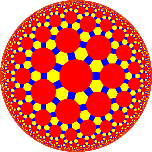
I bring this up (we’ll be ditching this picture in a sec) to show the basic reason that we are interested in modelling latent space as a hyperbolic space at all. The Tetradecagons within the hyperbolic space are of equal area.
Usually (in our Euclidean understanding of the world) as we move further out in space if you imagine the circle/sphere, area will increase as distance squared \(\pi r^2\) and volume distance cubed \(\frac{4}{3} \pi r^3\). In hyperbolic space though, the area and volume will increase exponentially!
This characteristic or quirk of the geometry lends itself to representing hierarchical or tree. It would make sense that data/categories may need to be represented with about the same amount of space in the latent space. i.e. no singular category/piece of data is any more or less complicated than any other.
Then as we increase the depth of the structure the amount of area needed to nicely represent te data exponentially increases. You can see this in the below two gifs.
So, similar to how linearly increasing the depth in the above tree exponentially increases the required width, in hyperbolic space linearly increasing distances exponentially increase area! So if you use a typical euclidean latent space you have to exponentially explore the space, which would be difficult for a neural network to model. So instead we will replace it with a hyperbolic space so that maybe the neural networks will only need to ‘linearly’ manoeuvre in the space.
For the rest of this post we will instead defer to the Lorentz/Hyperboloid/Minkowski model for hyperbolic space where basically we interpret N-dimensional hyperbolic space as a hyperboloid in \(\mathbb{R}^{N+1}\) with a Minkowski metric6 in a similar way to how we imagine spherical space to exist as sphere in \(\mathbb{R}^{N+1}\).
This model allows one to create the below ‘typical’ plot for observing how curvature manipulates the shapes representing the different spaces. The hyperboloid or what we will imagine as the hyperbolic the space exists for \(\kappa < 0\)7.
The more rigorous definition of the space \(\mathbb{H}^n\) is the set of points \(\vec{z} \in \mathbb{R}^{n+1}\) with \(z_0>0\) such that the Lorentzian inner product \(\langle ... \rangle_\mathcal{L}\), given as,
\[\begin{align} \langle \vec{z}^{(j)}, \vec{z}^{(k)} \rangle_\mathcal{L} = -z_0^{(j)} z_0^{(k)} + \sum_{i=1}^n z_i^{(j)} z_i^{(k)}, \end{align}\]is equal to \(-1\) if \(i=k\). i.e. \(\mathbb{H}^n = \{\vec{z} \in \mathbb{R}^{n+1} : \langle \vec{z}, \vec{z} \rangle_\mathcal{L} = -1, z_0>0 \}\). And like Nagano et al. (2019) we will use \(\vec{\mu}_0 = [1, 0, 0, ...] \in \mathbb{H}^n \subset \mathbb{R}^n\) as a kind of origin for the space.
Another fun thing about these spaces is how ‘straight lines’ behave and when I say ‘straight lines’ I mean geodesics. A practical definition for a geodesic is that it is the shortest path or set of points that connect to coordinates.
e.g. The ‘straight line’ or shortest path between two points on the sphere is curved. This can be seen in the diagram below showing different paths between Melbourne and Sapporo one of them is a little harder in practice. What one would think of as the ‘straight’ path isn’t really the straight path as it doesn’t exist in the spherical space. So the “actual” straight line is the curved line connecting the two points
Similarly, geodesics in hyperbolic space are not what we would call straight. Below are some examples of geodesics on/in the different geometries/spaces (this plot took me an embarassingly long time to make, please appreciate).

Another interesting thing is that unlike in Euclidean geometry, parallel lines don’t remain parallel! In essence, we can’t just explore this space will-nilly, we have to have some sort of map.
Tangent Space
Before we can even start navigating our maps though maybe we need some notion of direction. Let’s say we exist in the space of a sphere. We cannot view out into \(\mathbb{R}^3\) as it doesn’t exist to us, we can only see the geometry that is intrinsic to the space. So how do we ‘walk around’ if we don’t even know ‘where’ we can walk.
We define the ‘velocity’ vectors defining where we can move as existing in the Tangent Space. The Tangent Space for a given point on the manifold (\(\vec{\mu}\)), which we will denote \(T_\vec{\mu} \mathbb{H}^n\) for the hyperbolic space, can also be more simply thought of the space that contains the set tangent vectors in the same ambient space as the manifold \(\vec{u} \in \mathbb{R}^{n+1}\).
For the hyperbolic space we can define,
\[\begin{align} T_\vec{\mu} \mathbb{H}^n = \{\vec{u}: \langle \vec{u}, \vec{\mu}\rangle_\mathcal{L} = 0\}. \end{align}\]Which just ends up giving you lines and planes like the below.


Parallel Transport
Okay now that we have some notion of how to encode ‘direction’, now let’s figure out how to walk straight. In differential geometry we generalise the notion of ‘walking in a straight line’ into Parallel transport.
The parallel transport map is a rule for moving a vector along a curve from one point, \(p\), to another, \(q\), on a manifold. The key property is that the vector is translated such that it remains “constant” with respect to the geometry of the space (i.e., its intrinsic length and angle with respect to the curve are preserved).
More simply, it’s the process of sliding a vector along a curve without letting it rotate or change magnitude as it relates to the space’s local coordinates. If the curve you’re transporting the vector along is a geodesic, then the vector being parallel transported along that geodesic defines what a straight line looks like in that geometry.
e.g. If a vector is parallel to a geodesic we are travelling on (the generalised notion of a straight line) then it will remain parallel to the geodesic by the end.
Even more simply, in our usual Euclidean space, if I hold my arm out to the right and then walk in a straight line, unless I move it, my arm will still be to my right. However, let’s say that I’m a n-dimensional spherical being, and I’m on some positive latitude, if I hold my arm ‘up’ it will stay ‘up’ to me. But to some observer in \(\mathbb{R}^{n+1}\) it will initially look like I’m pointing ‘up and out’ but as I circle around, the observer will effectively see my arm reverse directions with respect to me. I’ve tried to visualise this below.
 from the perspective of \(\mathbb{R}^3\)")
 from the perspective of \(S^{2}\)")
The top vector/line isn’t a geodesic so the vector appears to rotate from both perspectives we show.
Because we are focused on the relative positions/directions of the vectors this mapping is defined between tangent spaces. So in hyperbolic space, if we have \(\vec{\mu}, \vec{\nu} \in \mathbb{H}^n\) then we define the parallel transport map that carries \(\vec{v} \in T_\vec{\nu}\mathbb{H}^n\) into \(\vec{u} \in T_\vec{\mu}\mathbb{H}^n\) as,
\[\begin{align} \vec{u} = \text{PT}_{\vec{\nu} \rightarrow \vec{\mu}}(\vec{v}) = \vec{v} + \frac{\langle \vec{\mu}-\alpha \vec{\nu}, \vec{v} \rangle_{\mathcal{L}}}{\alpha + 1}(\vec{\nu} + \vec{\mu}) \end{align}\]with \(\alpha = - \langle \vec{\mu}, \vec{\nu}\rangle_{\mathcal{L}}\). I’ve tried to recreate the gifs I made above for the sphere on the hyperbola, notably sans the perspective of the tangent space, because when I made the gif it wasn’t really clear what was going on anyway.
 from the perspective of \(\mathbb{R}^3\)")
 also from the perspective of \(\mathbb{R}^3\)")
It is also handy to have the inverse of this map, \(\text{PT}_{\vec{\nu}\rightarrow\vec{\mu}}^{-1}\), which maps the vectors in \(T_\vec{\mu}\mathbb{H}^n\) back to \(T_\vec{\nu}\mathbb{H}^n\), but that’s just parallel transport in the other direction.
\[\begin{align} \vec{v} = \text{PT}_{\vec{\nu}\rightarrow\vec{\mu}}^{-1}(\vec{u}) = \text{PT}_{\vec{\mu}\rightarrow\vec{\nu}}(\vec{v}) \end{align}\]The Exponential Map
So the above let’s us transport vectors between tangent spaces. Woop-de-doo. We want to generate samples on \(\mathbb{H}^n\) not on \(T_\vec{\mu}\mathbb{H}^n\) or \(T_\vec{\nu}\mathbb{H}^n\). What we need now is some way to map vectors \(\vec{\mu} \in \mathbb{H}^n\) and \(\vec{v} \in T_\vec{\mu}\mathbb{H}^n\). For the purpose of this work and Nagano et al. (2019) this will be fulfilled by the Exponential Map.
The exponential map connects linear structure, in the tangent space \(T_\vec{\mu} \mathbb{H}^n\) for example, to the manifold, e.g. \(\mathbb{H}^n\).
For a given \(\vec{\mu}\), the map finds the unique geodesic \(\gamma_{\vec{\mu}}(t)\) that starts at \(\vec{\mu}\) (i.e., \(\gamma_{\vec{\mu}}(0)=\vec{\mu}\)) and has \(\vec{v}\) as its initial velocity (i.e., \(\gamma_{\vec{\mu}}'(0)=\vec{v}\)).
The exponential map then simply evaluates this geodesic at \(t=1\): \(\exp_\vec{\mu}(\vec{v}) = \gamma_{\vec{v}}(1)\).
This setup is such that the magnitude \(\lVert\vec{v}\rVert\) of the input vector \(\vec{v}\) directly corresponds to the geodesic distance between the base point \(\vec{\mu}\) and the resulting point \(\exp_p(\vec{v})\), effectively using the tangent space as a “rolled out” local version of the manifold. This means that we can define samples in the tangent space of the “origin”, parallel transport them, then use the exponential map to map these transported samples onto the hyperbolic manifold.
For the n-dimensional hyperbolic space we define the exponential map for \(\vec{\mu} \in \mathbb{H}^n\) and \(\vec{u} \in T_\vec{\mu} \mathbb{H}^n\) as,
\[\begin{align} \vec{v} = \exp_\vec{\mu}(\vec{u}) = \cosh\left(\lVert \vec{u} \rVert_\mathcal{L}\right) \vec{\mu} + \sinh\left(\lVert \vec{u} \rVert_\mathcal{L}\right) \frac{\vec{u}}{\lVert \vec{u} \rVert_\mathcal{L}}. \end{align}\]The map is also norm preserving meaning that,
\[\begin{align} &d_\mathcal{L}(\vec{\mu}, \exp_\vec{\mu}(\vec{u})) \\ &= \text{arccosh}\left(-\langle \vec{\mu}, \exp_\vec{\mu}(\vec{u}) \rangle_\mathcal{L} \right) \\ &= \text{arccosh}\left(-\langle \vec{\mu}, \cosh\left(\lVert \vec{u} \rVert_\mathcal{L}\right) \vec{\mu} + \sinh\left(\lVert \vec{u} \rVert_\mathcal{L}\right) \frac{\vec{u}}{\lVert \vec{u} \rVert_\mathcal{L}} \rangle_\mathcal{L} \right) \\ &= \text{arccosh}\left(-\cosh\left(\lVert \vec{u} \rVert_\mathcal{L}\right) \langle \vec{\mu}, \vec{\mu}\rangle_\mathcal{L} + \sinh\left(\lVert \vec{u} \rVert_\mathcal{L}\right) \frac{1}{\lVert \vec{u} \rVert_\mathcal{L}} \langle \vec{\mu},\vec{u} \rangle_\mathcal{L} \right) \\ &= \text{arccosh}\left(-\cosh\left(\lVert \vec{u} \rVert_\mathcal{L}\right) \cdot (-1) + \sinh\left(\lVert \vec{u} \rVert_\mathcal{L}\right) \frac{1}{\lVert \vec{u} \rVert_\mathcal{L}} \cdot 0\right) \\ &= \text{arccosh}\left(\cosh\left(\lVert \vec{u} \rVert_\mathcal{L}\right)\right) \\ \\ &d_\mathcal{L}(\vec{\mu}, \exp_\vec{\mu}(\vec{u})) = \lVert \vec{u} \rVert_\mathcal{L} \end{align}\]And of course we like having the inverse,
\[\begin{align} \vec{u} = \exp_\vec{\mu}^{-1}(\vec{v}) = \frac{\text{arccosh}(\alpha)}{\sqrt{\alpha^2 - 1}} (\vec{v} - \alpha \vec{\mu}), \end{align}\]with \(\alpha = -\langle \vec{\mu}, \vec{v}\rangle_\mathcal{L}\) again.
Below is a visualisations showing how the mapping morphs the tangent space on to a neighbourhood of \(\mathbb{H}^n\) around \(\vec{\mu}\).
 into \(\mathbb{H}^{2}\).")
The Pseudo-Hyperbolic Gaussian or Wrapped Normal Distribution on Hyperbolic Space
We are now done with the hard stuff. From here’s it’s real simple. We just need to do two things:
- Figure out how to sample a projected normal distribution in hyperbolic space (easier than it sounds)
- How to evaluate the density
1. Sampling the Pseudo-Hyperbolic Gaussian
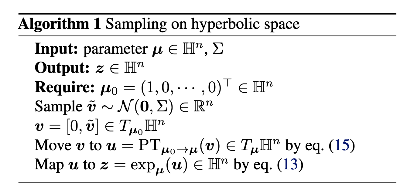
The way Nagano et al. (2019) sample what they call a ‘wrapped’ gaussian distribution \(\mathcal{G}(\vec{\mu}, \Sigma)\) for a mean coordinate \(\vec{\mu} \in \mathbb{H}^n\) is simply:
- Sample \(\vec{v}' \sim \mathcal{N}(\vec{0}, \Sigma) \in \mathbb{R}^n\)
- Set \(\vec{v} = [0, \vec{v}']\) such that \(\vec{v} \in T_{\vec{\mu}_0}\mathbb{H}^n\) (remembering that \(\vec{\mu}_0\) defined our ‘origin’ and can be interpreted as the bottom of the hyperboloid, where the vertical direction corresponds to the first dimension)
- Us parallel transport to move the samples in the tangent space \(\vec{v} \in T_{\vec{mu}_0}\mathbb{H}^n\) into the tangent space \(\vec{u} \in T_{\vec{\mu}}\mathbb{H}^n\) (along the relevant geodesic/straight line)
- Use the exponential map \(\exp_\vec{\mu}\) to map the samples in \(T_{\vec{\mu}}\mathbb{H}^n\) on to \(\mathbb{H}^n\)
And that’s it. The beauty of this is that it also allows us to easily perform the reparameterisation trick, as we can sample \(\epsilon\) in the first step to capture the stochasticity!
I demonstrate the general process in the case of \(\mathbb{H}^1\) in the gifs below.


I will also directly copy-paste the algorithm directly from Nagano et al. (2019) below as well.
2. Evaluating the Pseudo-Hyperbolic Gaussian density
We can sample the distribution, now we want to figure out the density of the projected distribution/the probabilities of samples in \(\mathbb{H}^n\). To do this we use the typical formula for the pushforward of a density,
\[\begin{align} \log p(\vec{z}) = \log p(\vec{v}) - \log \det \left(\frac{\partial f}{\partial \vec{v}} \right). \end{align}\]In our case \(f\) is the transformation of the samples from the tangent space of \(\vec{\mu}_0\) to \(\mathbb{H}^n\) around \(\vec{\mu}\), that is \(f = \exp_\vec{\mu} \circ \text{PT}_{\vec{\mu}_0 \rightarrow \vec{\mu}}\).
By the chain rule,
\[\begin{align} &\det \left(\frac{\partial}{\partial \vec{v}} \exp_\vec{\mu} \circ \text{PT}_{\vec{\mu}_0 \rightarrow \vec{\mu}} \right) \\ &= \det \left( \frac{\partial}{\partial \vec{u}} \exp_\vec{\mu}(\vec{u}) \cdot \frac{\partial}{\partial \vec{v}} \text{PT}_{\vec{\mu}_0 \rightarrow \vec{\mu}}(\vec{v}) \right)\\ &= \det \left( \frac{\partial}{\partial \vec{u}} \exp_\vec{\mu}(\vec{u})\right) \cdot \det \left(\frac{\partial}{\partial \vec{v}} \text{PT}_{\vec{\mu}_0 \rightarrow \vec{\mu}}(\vec{v}) \right) \end{align}\]Now just for completeness I’m going to include the derivations for both of these, but there’s nothing much to add that isn’t already in Appendix A.3 and A.4 in Nagano et al. (2019). Which is a good reminder that if you do feel so inclined to ever cite me, please always cite the work that I’m likely referencing and you may find that you don’t need to cite me at all anyways.
\(\det \left( \frac{\partial}{\partial \vec{u}} \exp_\vec{\mu}(\vec{u})\right)\) Derivation
For this derivation we will use an orthonormal basis such that the determinant is simply the product of the individual directional derivatives for each basis. Additionally, we will construct that basis such that the first component is the unit vector in the direction of \(\vec{u}\), \(\bar{u} = \vec{u}/\lVert \vec{u}\rVert_\mathcal{L} = \vec{u}/r\). This means for the basis \(\{\bar{u}=\vec{u}_1', \vec{u}_2', \vec{u}_3',...\}\) where \(\lVert \vec{u}_k'\rVert_\mathcal{L}=1\) and \(\langle \vec{u}_i',\vec{u}_k'\rangle_\mathcal{L} = \delta_{ik}\),
\[\begin{align} \det \left( \frac{\partial}{\partial \vec{u}} \exp_\vec{\mu}(\vec{u})\right) = \prod_{i=1}^n \left\lVert \frac{\partial}{\partial \vec{u}_i'} \exp_\vec{\mu}(\vec{u})\right\rVert_\mathcal{L}. \end{align}\]We then have two cases of where \(\vec{u}_k'\) equals \(\bar{u}\) or not.
\[\begin{align} \frac{\partial}{\partial \bar{u}} \exp_\vec{\mu}(\vec{u}) &= \frac{d}{d\epsilon}\big\vert_{\epsilon=0} \left(\cosh\left(\lVert \vec{u} + \epsilon \bar{u} \rVert_\mathcal{L}\right) \vec{\mu} + \sinh\left(\lVert \vec{u} + \epsilon \bar{u} \rVert_\mathcal{L}\right) \frac{\vec{u} + \epsilon \bar{u}}{\lVert \vec{u} + \epsilon \bar{u}\rVert_\mathcal{L}} \right) \\ &= \frac{d}{d\epsilon}\big\vert_{\epsilon=0} \left(\cosh\left(\lVert (r + \epsilon) \bar{u} \rVert_\mathcal{L}\right) \vec{\mu} + \sinh\left(\lVert (r + \epsilon) \bar{u} \rVert_\mathcal{L}\right) \frac{(r + \epsilon) \bar{u}}{\lVert (r + \epsilon) \bar{u}\rVert_\mathcal{L}} \right) \\ &= \frac{d}{d\epsilon}\big\vert_{\epsilon=0} \left(\cosh\left(r + \epsilon \right) \vec{\mu} + \sinh\left(r + \epsilon\right) \bar{u} \right)\\ &= \left(\sinh\left(r + \epsilon \right) \vec{\mu} + \cosh\left(r + \epsilon\right) \bar{u} \right) \big\vert_{\epsilon=0} \\ &= \sinh\left(r \right) \vec{\mu} + \cosh\left(r\right) \bar{u} \end{align}\]With,
\[\begin{align} &\langle \sinh\left(r \right) \vec{\mu} + \cosh\left(r\right) \bar{u}, \sinh\left(r \right) \vec{\mu} + \cosh\left(r\right) \bar{u}\rangle_{\mathcal{L}} \\ &= \sinh\left(r \right)^2 \langle \vec{\mu}, \vec{\mu} \rangle_\mathcal{L} + 2\cosh\left(r\right)\sinh\left(r \right) \langle \vec{\mu}, \bar{u}\rangle_\mathcal{L} + \cosh\left(r\right)^2 \langle \vec{u}, \bar{u}\rangle_{\mathcal{L}} \\ &= \sinh\left(r \right)^2 \cdot (-1) + 2\cosh\left(r\right)\sinh\left(r \right) \cdot 0 + \cosh\left(r\right)^2 \cdot 1\\ &= \cosh\left(r\right)^2 - \sinh\left(r \right)^2 = 1. \end{align}\]And before the next bit I’ll just say that
\[\begin{align} \lVert \vec{u} + \epsilon \vec{u}_k' \rVert_\mathcal{L} &= \sqrt{\langle \vec{u}, \vec{u}\rangle_\mathcal{L} + \epsilon \langle \vec{u}, \vec{u}_k'\rangle_\mathcal{L} + \epsilon^2 \langle \vec{u}_k', \vec{u}_k'\rangle_\mathcal{L} \langle } \\ &= \sqrt{r^2 + \epsilon \cdot 0 + \epsilon^2 \cdot 1 } \\ &= \sqrt{r^2 + \epsilon^2 }, \\ \end{align}\]and \(\frac{d}{d\epsilon} \sqrt{r^2 + \epsilon^2 } = \frac{\epsilon}{\sqrt{r^2 + \epsilon^2}}\).
Using this,
\[\begin{align} \frac{\partial}{\partial \vec{u}_{k\neq 1}'} \exp_\vec{\mu}(\vec{u}) &= \frac{d}{d\epsilon}\big\vert_{\epsilon=0} \left(\cosh\left(\lVert \vec{u} + \epsilon \vec{u}_k' \rVert_\mathcal{L}\right) \vec{\mu} + \sinh\left(\lVert \vec{u} + \epsilon \vec{u}_k' \rVert_\mathcal{L}\right) \frac{\vec{u} + \epsilon \vec{u}_k' }{\lVert \vec{u} + \epsilon \vec{u}_k' \rVert_\mathcal{L}} \right) \\ &= \frac{d}{d\epsilon}\big\vert_{\epsilon=0} \left(\cosh\left(\sqrt{r^2 + \epsilon^2 }\right) \vec{\mu} + \sinh\left(\sqrt{r^2 + \epsilon^2 }\right) \frac{\vec{u} + \epsilon \vec{u}_k' }{\sqrt{r^2 + \epsilon^2 }} \right) \\ &= \left[ \frac{\epsilon}{\sqrt{r^2 + \epsilon^2}} \sinh\left(\sqrt{r^2 + \epsilon^2 }\right) \vec{\mu} \color{white} \right] \color{black} \\ &\;\;\;\;\;\;+ \color{white} \color{black} \frac{\epsilon}{\sqrt{r^2 + \epsilon^2}} \cosh\left(\sqrt{r^2 + \epsilon^2 }\right) \frac{\vec{u} + \epsilon \vec{u}_k' }{\sqrt{r^2 + \epsilon^2 }} \\ &\;\;\;\;\;\;+ \color{white} \left[ \color{black} \sinh\left(\sqrt{r^2 + \epsilon^2 }\right) \left( \frac{\vec{u}_k' }{\sqrt{r^2 + \epsilon^2 }} - \frac{\epsilon\vec{u} + \epsilon^2 \vec{u}_k' }{\sqrt{(r^2 + \epsilon^2)^3 }} \right) \right] \color{black} {\Huge\vert}_{\epsilon=0} \\ &= \frac{\sinh\left(r\right)}{r} \vec{u}_k'\\ \end{align}\]With \(\lVert \frac{\sinh\left(r\right)}{r} \vec{u}_k' \rVert_\mathcal{L} = \frac{\sinh\left(r\right)}{r} \lVert\vec{u}_k'\rVert_\mathcal{L} = \frac{\sinh\left(r\right)}{r}\) due to our choice of basis. Hence,
\[\begin{align} \det \left( \frac{\partial}{\partial \vec{u}} \exp_\vec{\mu}(\vec{u})\right) = \left(\frac{\sinh\left(r\right)}{r} \right)^{n-1} \end{align}\]\(\det \left(\frac{\partial}{\partial \vec{v}} \text{PT}_{\vec{\mu}_0 \rightarrow \vec{\mu}}(\vec{v})\right)\) Derivation
Then for \(\vec{v} \in T_{\vec{\mu}_0} \mathbb{H}^n\) and any ol’ relevant orthonormal basis \(\{\vec{\xi}_1,\vec{\xi}_2, \vec{\xi}_3,..\}\) and \(\alpha = -\langle \vec{\mu}_0, \vec{\mu}\rangle_\mathcal{L}\),
\[\begin{align} \frac{\partial}{\partial \vec{\xi}_k} \text{PT}_{\vec{\mu}_0 \rightarrow \vec{\mu}}(\vec{v}) &= \frac{\partial}{\partial \epsilon} \lvert_{\epsilon=0} \text{PT}_{\vec{\mu}_0 \rightarrow \vec{\mu}}(\vec{v} + \epsilon \vec{\xi}_k) \\ &= \frac{\partial}{\partial \epsilon} \lvert_{\epsilon=0} \left( (\vec{v} + \epsilon \vec{\xi}_k) + \frac{\langle \vec{\mu} - \alpha \vec{\mu}_0, (\vec{v} + \epsilon \vec{\xi}_k) \rangle_\mathcal{L}}{\alpha + 1} \left(\vec{\mu}_0 +\vec{\mu} \right) \right)\\ &= \vec{\xi}_k + \frac{\partial}{\partial \epsilon} \left( \frac{\langle \vec{\mu} - \alpha \vec{\mu}_0, \vec{v} \rangle_\mathcal{L} + \epsilon \langle \vec{\mu} - \alpha \vec{\mu}_0, \vec{\xi}_k \rangle_\mathcal{L}}{\alpha + 1} \left(\vec{\mu}_0 +\vec{\mu} \right) \right)\lvert_{\epsilon=0} \\ &= \vec{\xi}_k + \frac{\langle \vec{\mu} - \alpha \vec{\mu}_0, \vec{\xi}_k \rangle_\mathcal{L}}{\alpha + 1} \left(\vec{\mu}_0 +\vec{\mu} \right) \\ &= \text{PT}_{\vec{\mu}_0 \rightarrow \vec{\mu}}(\vec{\xi}_k) \end{align}\]The parallel transport map is then norm preserving, meaning that \(\lVert \text{PT}_{\vec{\mu}_0 \rightarrow \vec{\mu}}(\vec{\xi}_k) \rVert_\mathcal{L} = 1\). This makes sense as it’s basically the generalisation of what happens after walking in a straight line in Euclidean space, you wouldn’t expect your arm to grow just because you walk a few steps. But we can also show this algebraically if that analogy isn’t satisfactory (I said before realising how muh algebra was needed and why Nagano et al. (2019) skipped it…),
\[\begin{align} & \langle \text{PT}_{\vec{\mu}_0 \rightarrow \vec{\mu}}(\vec{\xi}_k), \text{PT}_{\vec{\mu}_0 \rightarrow \vec{\mu}}(\vec{\xi}_k)\rangle_\mathcal{L} \\ &= \langle \vec{\xi}_k + \frac{\langle \vec{\mu} - \alpha \vec{\mu}_0, \vec{\xi}_k \rangle_\mathcal{L}}{\alpha + 1} \left(\vec{\mu}_0 +\vec{\mu} \right), \vec{\xi}_k + \frac{\langle \vec{\mu} - \alpha \vec{\mu}_0, \vec{\xi}_k \rangle_\mathcal{L}}{\alpha + 1} \left(\vec{\mu}_0 +\vec{\mu} \right) \rangle_\mathcal{L}\\ &= \langle \vec{\xi}_k, \vec{\xi}_k\rangle_\mathcal{L} + \frac{\langle \vec{\mu} - \alpha \vec{\mu}_0, \vec{\xi}_k \rangle_\mathcal{L}}{\alpha + 1} \langle \vec{\xi}_k,\left(\vec{\mu}_0 +\vec{\mu} \right)\rangle_\mathcal{L} + \left(\frac{\langle \vec{\mu} - \alpha \vec{\mu}_0, \vec{\xi}_k \rangle_\mathcal{L}}{\alpha + 1}\right)^2 \langle \left(\vec{\mu}_0 +\vec{\mu} \right),\left(\vec{\mu}_0 +\vec{\mu} \right)\rangle_\mathcal{L}\\ \end{align}\]Letting \(C = \frac{\langle \vec{\mu} - \alpha \vec{\mu}_0, \vec{\xi}_k \rangle_\mathcal{L}}{\alpha + 1}\)
\[\begin{align} & \langle \text{PT}_{\vec{\mu}_0 \rightarrow \vec{\mu}}(\vec{\xi}_k), \text{PT}_{\vec{\mu}_0 \rightarrow \vec{\mu}}(\vec{\xi}_k)\rangle_\mathcal{L} \\ &= \langle \vec{\xi}_k, \vec{\xi}_k\rangle_\mathcal{L} + C \langle \vec{\xi}_k,\left(\vec{\mu}_0 +\vec{\mu} \right)\rangle_\mathcal{L} + C^2 \langle \left(\vec{\mu}_0 +\vec{\mu} \right),\left(\vec{\mu}_0 +\vec{\mu} \right)\rangle_\mathcal{L}\\ \end{align}\]Splitting this into bits (remembering that \(\vec{\xi}_k\) is a basis for the inputs \(\vec{v} \in T_{\vec{\mu}_0}\mathbb{H}^n\)),
\[\begin{align}\langle \vec{\xi}_k,\left(\vec{\mu}_0 +\vec{\mu} \right)\rangle_\mathcal{L} \\ = \langle \vec{\xi}_k, \vec{\mu}_0\rangle_\mathcal{L} + \langle \vec{\xi}_k,\vec{\mu} \rangle_\mathcal{L}\\ = \langle \vec{\xi}_k,\vec{\mu} \rangle_\mathcal{L}\\ \end{align}\]And similarly,
\[\begin{align} C &= \frac{\langle \vec{\mu} - \alpha \vec{\mu}_0, \vec{\xi}_k \rangle_\mathcal{L}}{\alpha + 1} \\ &= \frac{\langle \vec{\mu}, \vec{\xi}_k \rangle_\mathcal{L} - \alpha \langle \vec{\mu}_0, \vec{\xi}_k \rangle_\mathcal{L}}{\alpha + 1} \\ &= \frac{\langle \vec{\mu}, \vec{\xi}_k \rangle_\mathcal{L}}{\alpha + 1}. \\ \end{align}\]And finally,
\[\begin{align} &\langle \left(\vec{\mu}_0 +\vec{\mu} \right),\left(\vec{\mu}_0 +\vec{\mu} \right)\rangle_\mathcal{L} \\ &=\langle \vec{\mu}_0,\vec{\mu}_0 \rangle_\mathcal{L} + 2\langle \vec{\mu}_0, \vec{\mu}\rangle_\mathcal{L} + \langle \vec{\mu}, \vec{\mu} \rangle_\mathcal{L} \\ &= -1 - 2 \alpha - 1\\ &= -2 (1 + \alpha) \\ \end{align}\]Now we can put it all back together again,
\[\begin{align} & \langle \text{PT}_{\vec{\mu}_0 \rightarrow \vec{\mu}}(\vec{\xi}_k), \text{PT}_{\vec{\mu}_0 \rightarrow \vec{\mu}}(\vec{\xi}_k)\rangle_\mathcal{L} \\ &= \langle \vec{\xi}_k, \vec{\xi}_k\rangle_\mathcal{L} + C \langle \vec{\xi}_k,\left(\vec{\mu}_0 +\vec{\mu} \right)\rangle_\mathcal{L} + C^2 \langle \left(\vec{\mu}_0 +\vec{\mu} \right),\left(\vec{\mu}_0 +\vec{\mu} \right)\rangle_\mathcal{L}\\ &= \langle \vec{\xi}_k, \vec{\xi}_k\rangle_\mathcal{L} + \frac{\langle \vec{\mu}, \vec{\xi}_k \rangle_\mathcal{L}^2}{\alpha + 1} - 2 (1 + \alpha) \left(\frac{\langle \vec{\mu}, \vec{\xi}_k \rangle_\mathcal{L}}{\alpha + 1}\right)^2 \\ &= \langle \vec{\xi}_k, \vec{\xi}_k\rangle_\mathcal{L} + \frac{\langle \vec{\mu}, \vec{\xi}_k \rangle_\mathcal{L}^2}{\alpha + 1} - 2 \frac{\langle \vec{\mu}, \vec{\xi}_k \rangle_\mathcal{L}^2}{\alpha + 1} \\ &= \langle \vec{\xi}_k, \vec{\xi}_k\rangle_\mathcal{L} = 1. \end{align}\]In Summary
\[\begin{align} \log p(\vec{z}) = \log \mathcal{N}(\text{PT}_{\vec{\mu} \rightarrow \vec{\mu}_0}(\exp_\vec{\mu}^{-1}(\vec{z})) | \vec{0}, \Sigma) - (n-1) \log \left(\frac{\sinh\left(\lVert\exp_\vec{\mu}^{-1}(\vec{z}) \rVert_\mathcal{L} \right)}{\lVert \exp_\vec{\mu}^{-1}(\vec{z}) \rVert_\mathcal{L}} \right). \end{align}\]Putting the hyperbolic into the VAE
So in the case of the VAE we have our ‘gaussian’ distribution where we can learn the mean and the variance \(\mathcal{G}(\vec{\mu}, \Sigma)\), and \(\mathcal{G}(\vec{\mu}_0, \mathbb{I})\) works as the prior on that space. I didn’t make the mistake of looking for a GitHub page that had already implemented this beforehand, so if my code is similar to yours, it should be a coincidence.
Anyways, we need to do four things8:
1.Encode our base transformations (PT, exponential map, Lorentz product, etc)
import torch


def lorentz_inner_product(x, y):
    # -x0*y0 + x1*y1 + ... + xn*yn
    return -x[..., 0] * y[..., 0] + torch.sum(x[..., 1:] * y[..., 1:], dim=-1)

def lorentz_norm_sq(x):
    #||x||_L^2 = <x, x>_L
    return lorentz_inner_product(x, x)

def lorentz_norm(x):
    #||x||_L = sqrt(<x, x>_L)
    return torch.sqrt(lorentz_norm_sq(x))

def exp_map(mu, u):
    # T_\mu(\mathbb{H}^n) -> H^n
    r = lorentz_norm(u)

    # making sure that r isn't too small, making everything explode # not great
    epsilon = 1e-6
    return torch.cosh(r).unsqueeze(-1) * mu + torch.sinh(r).unsqueeze(-1) * (u / r.unsqueeze(-1).clamp(min=epsilon))

def inv_exp_map(mu, z):
    # exp_mu^{-1}(z) : H^n -> T_mu(H^n)
    alpha = -lorentz_inner_product(mu, z) # alpha = cosh(d(mu, z))

    # Similar thing to r above
    alpha = torch.clamp(alpha, min=1.0)

    d = torch.acosh(alpha)

    # Clampin
    sinh_d = torch.sqrt(alpha**2 - 1).clamp(min=1e-6)

    u = (d / sinh_d).unsqueeze(-1) * (z - alpha.unsqueeze(-1) * mu)
    return u

def parallel_transport(nu, mu, v):
    # PT_{x->y}(v) : T_nu(H^n) -> T_mu(H^n)
    alpha = -lorentz_inner_product(nu, mu)

    # Clampin
    alpha = torch.clamp(alpha, min=1.0)

    # c = <y - alpha*x, v>_L / (1 + alpha)
    # y_minus_alpha_x = y - alpha*x
    # c = <y_minus_alpha_x, v>_L / (1 + alpha)
    numerator = lorentz_inner_product(mu - alpha.unsqueeze(-1) * nu, v)
    denominator = 1.0 + alpha

    c = (numerator / denominator).unsqueeze(-1)

    # PT(v) = v + c * (x + y)
    return v + c * (nu + mu)
2.Sample the wrapped gaussian and evaluate it’s density (kinda the reverse of the sampling)
def sample_wrapped_gaussian(mu, log_sigma, epsilon):
    # For my sanity we'll assume a diagonal covariance matrix
    sigma = torch.diag_embed(torch.exp(log_sigma)) # (batch x n x n)
    L = torch.linalg.cholesky(sigma) # (batch x n x n)

    # Assumes epsilon is already sampled and is size (b x n)

    # (b x n)
    v_prime = torch.bmm(L, epsilon.unsqueeze(-1)).squeeze(-1)

    # Chucking the zeros in the first dim so that are samples are in the tangent space
        # the 'centre' $$\vec{\mu_0}$$
    mu_0 = torch.zeros_like(mu)
    mu_0[:, 0] = 1.0 # (batch x n+1)
    v = torch.cat([torch.zeros_like(mu[:, 0]).unsqueeze(-1), v_prime], dim=-1) # (batch x n+1)

    # Then PT --> exp
    u = parallel_transport(mu_0, mu, v) # (batch x n+1)
    z = exp_map(mu, u) # (batch x n+1)

    # Also gonna return u so we can immediately use it for density estimation
        # and don't waste time converting z back into u
    return z, u


def log_prob_wrapped_gaussian(z, mu, log_sigma, n_dim):
    u = inv_exp_map(mu, z) # (batch x n+1)

    mu_0 = torch.zeros_like(mu)
    mu_0[:, 0] = 1.0
    v = parallel_transport(mu, mu_0, u) # (batch x n+1)

    # (batch x n)
    v_prime = v[:, 1:]

    log_2pi_term = n_dim * torch.log(torch.tensor(2.0 * torch.pi, device=z.device))
    log_det_sigma = torch.sum(log_sigma, dim=-1) # (batch,)

    a_sq = torch.sum(v_prime**2 * torch.exp(-log_sigma), dim=-1) # (batch,)

    log_N = -0.5 * (log_2pi_term + log_det_sigma + a_sq) # (batch,)

    # Calculating the Log Jacobian
    r = lorentz_norm(u) # (batch)
    r_clamped = torch.clamp(r, min=1e-6) # Clampin
    log_sinh_r_over_r = torch.log(torch.sinh(r_clamped) / r_clamped)

    log_det_J = (n_dim - 1) * log_sinh_r_over_r # (batch)

    # And finally, we get the thing. I know very detailed.
    log_p_z = log_N - log_det_J # (batch)

    return log_p_z
3.Evaluate the KL divergence term in the loss (same as the usual VAE)
def kl_divergence_wrapped_gaussian(mu_q, log_sigma_q, n_dim):
    # Sigma_q = diag(exp(log_sigma_q))
    sigma_q = torch.exp(log_sigma_q) # (batch x n)

    # tr(Sigma_q)
    tr_sigma_q = torch.sum(sigma_q, dim=-1) # (batch)

    # d(mu_q, mu_0)^2
    mu_0 = torch.zeros_like(mu_q)
    mu_0[:, 0] = 1.0

    alpha = -lorentz_inner_product(mu_q, mu_0) # alpha = cosh(d(mu_q, mu_0))
    alpha = torch.clamp(alpha, min=1.0)

    # d(mu_q, mu_0) = arccosh(alpha)
    distance_sq = torch.acosh(alpha)**2 # (batch)

    # -log det(Sigma_q) = -sum(log_sigma_q)
    log_det_sigma_q = torch.sum(log_sigma_q, dim=-1) # (batch)

    # KL = 0.5 * [tr(Sigma_q) + d(mu_q, mu_0)^2 - n - log det(Sigma_q)]
    kl_div = 0.5 * (tr_sigma_q + distance_sq - n_dim - log_det_sigma_q)

    return kl_div # (batch)
4.Chuck this all into a VAE. We’ll structure it so that there is some central ‘encoder’ fc1_enc and then using that we’ll have two smaller neural networks that will learn the mean and variances fc_mu and fc_logsigma (log to ensure positivity) and then a two layer decoder.
import torch
import torch.nn as nn
import torch.optim as optim
from torch.utils.data import DataLoader
from torchvision import datasets, transforms
import torch.nn.functional as F


class HVAE(nn.Module):
    def __init__(self, input_dim=784, hidden_dim=400, latent_dim=2):
        super().__init__()
        self.latent_dim = latent_dim
        self.n_dim = latent_dim  # The latent space dimension n

        #encoder
        self.fc1_enc = nn.Linear(input_dim, hidden_dim)

        self.fc_mu = nn.Linear(hidden_dim, latent_dim + 1)

        self.fc_logsigma = nn.Linear(hidden_dim, latent_dim)

        #dencoder
        self.fc1_dec = nn.Linear(latent_dim + 1, hidden_dim)
        self.fc2_dec = nn.Linear(hidden_dim, input_dim)

    def encode(self, x):
        h = F.relu(self.fc1_enc(x))
        mu_raw = self.fc_mu(h)
        log_sigma = self.fc_logsigma(h)

        mu_norm_sq = torch.sum(mu_raw[:, 1:]**2, dim=-1, keepdim=True)
        mu_0 = torch.sqrt(1 + mu_norm_sq)
        mu = torch.cat([mu_0, mu_raw[:, 1:]], dim=-1)

        return mu, log_sigma

    def decode(self, z):
        h = F.relu(self.fc1_dec(z))
        x_recon = torch.sigmoid(self.fc2_dec(h))
        return x_recon

    def forward(self, x):
        # Flatten
        x = x.view(x.size(0), -1)

        mu_q, log_sigma_q = self.encode(x)

        # reparameterization trick
        epsilon = torch.randn_like(log_sigma_q)

        z, u_q = sample_wrapped_gaussian(mu_q, log_sigma_q, epsilon)

        x_recon = self.decode(z)

        return x_recon, mu_q, log_sigma_q

    def loss_function(self, x_recon, x, mu_q, log_sigma_q):
        # flatten input
        x = x.view(x.size(0), -1)

        RE = F.binary_cross_entropy(x_recon, x, reduction='sum') / x.size(0)

        KL_H = kl_divergence_wrapped_gaussian(mu_q, log_sigma_q, self.n_dim)

        KL_H = torch.mean(KL_H)

        ELBO_loss = RE + KL_H

        return ELBO_loss, RE, KL_H
Image Classification and Generation for MNIST and LFW with constant curvature VAEs
Okay, so we (finally) have everything coded up and working (because I’ve run this beforehand). Let’s compare the performance of the Spherical VAE (SVAE), the standard VAE or ‘Euclidean’ VAE (EVAE) and hyperbolic VAE (HVAE) on some image data.
MNIST
To start off with let’s look at how the different VAEs tackle MNIST data with a 2D dimension latent dimension (meaning that the latent space manifold is two dimensional) with 2 layered neural networks with 128 nodes in the hiddens layers.
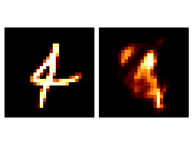
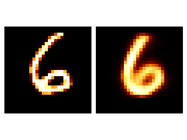
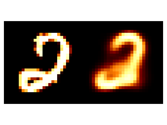
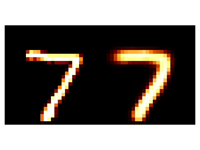
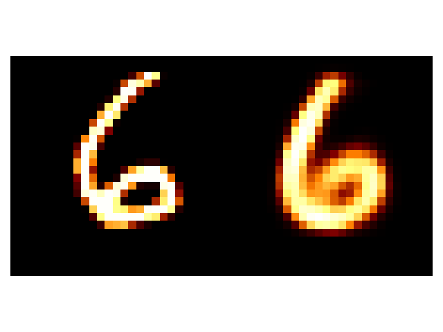
Let’s first see how well the different methods reconstruct different inputs.
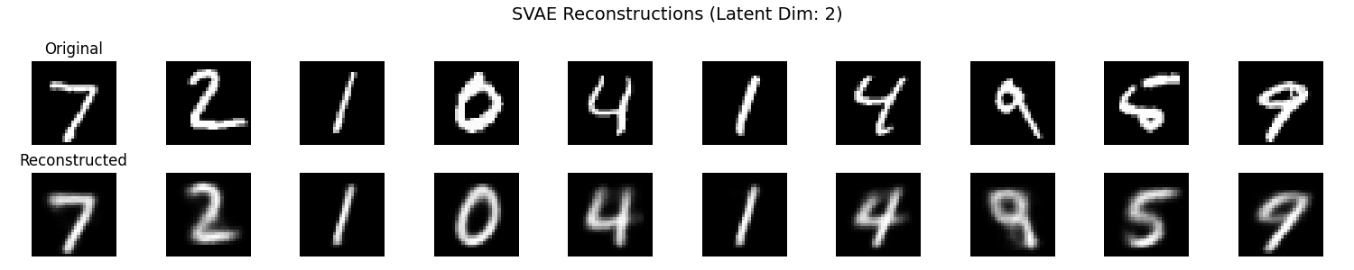

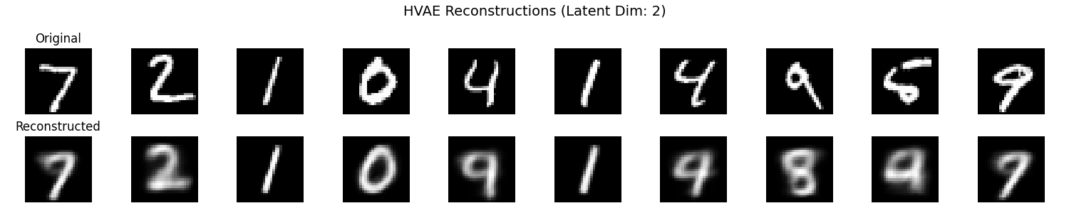
It seems that the SVAE did the best and HVAE did the worst, but this may just be because of the varying implementations. I’ll do a more quantitative comparison after some fun visuals.
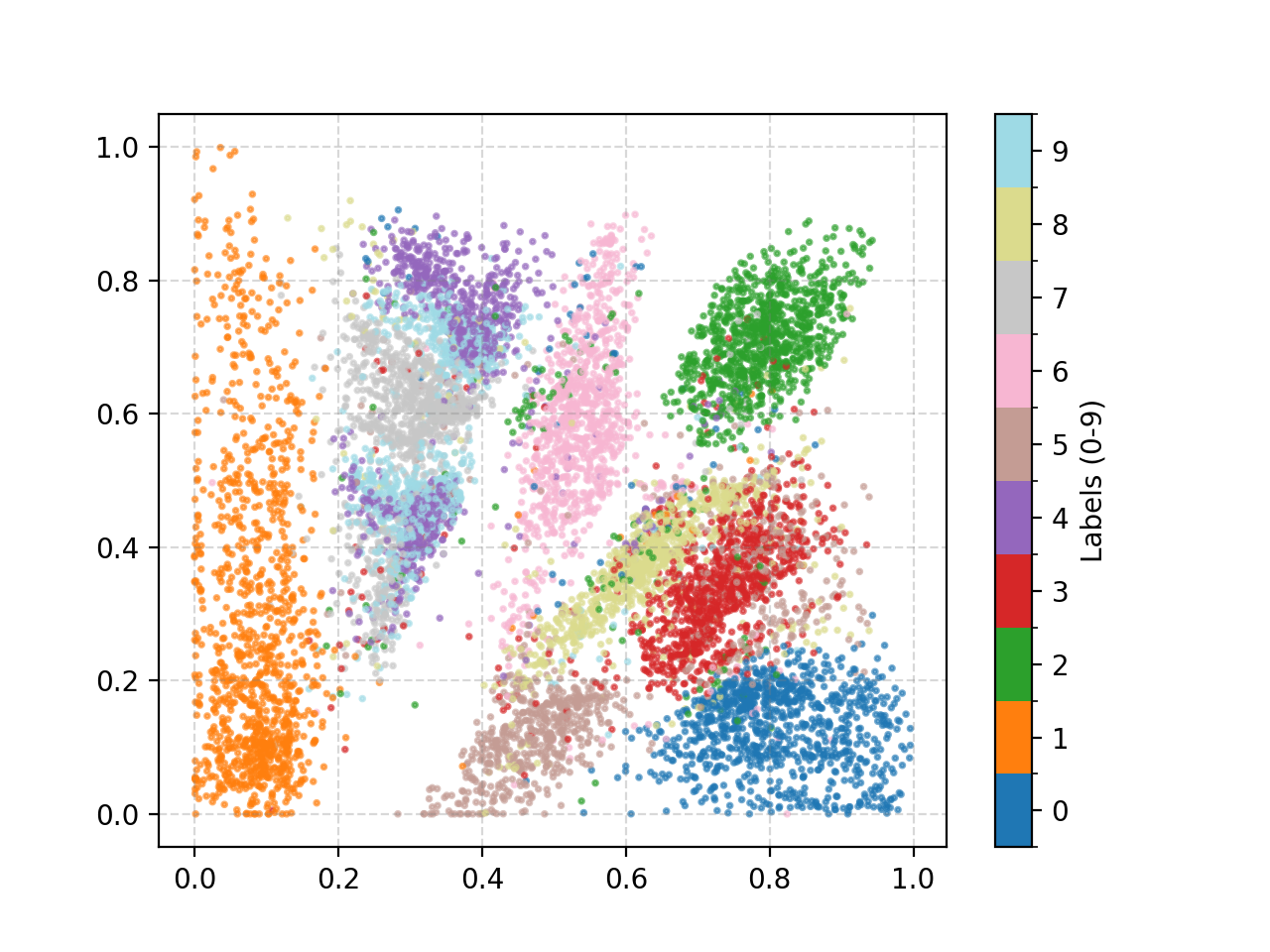
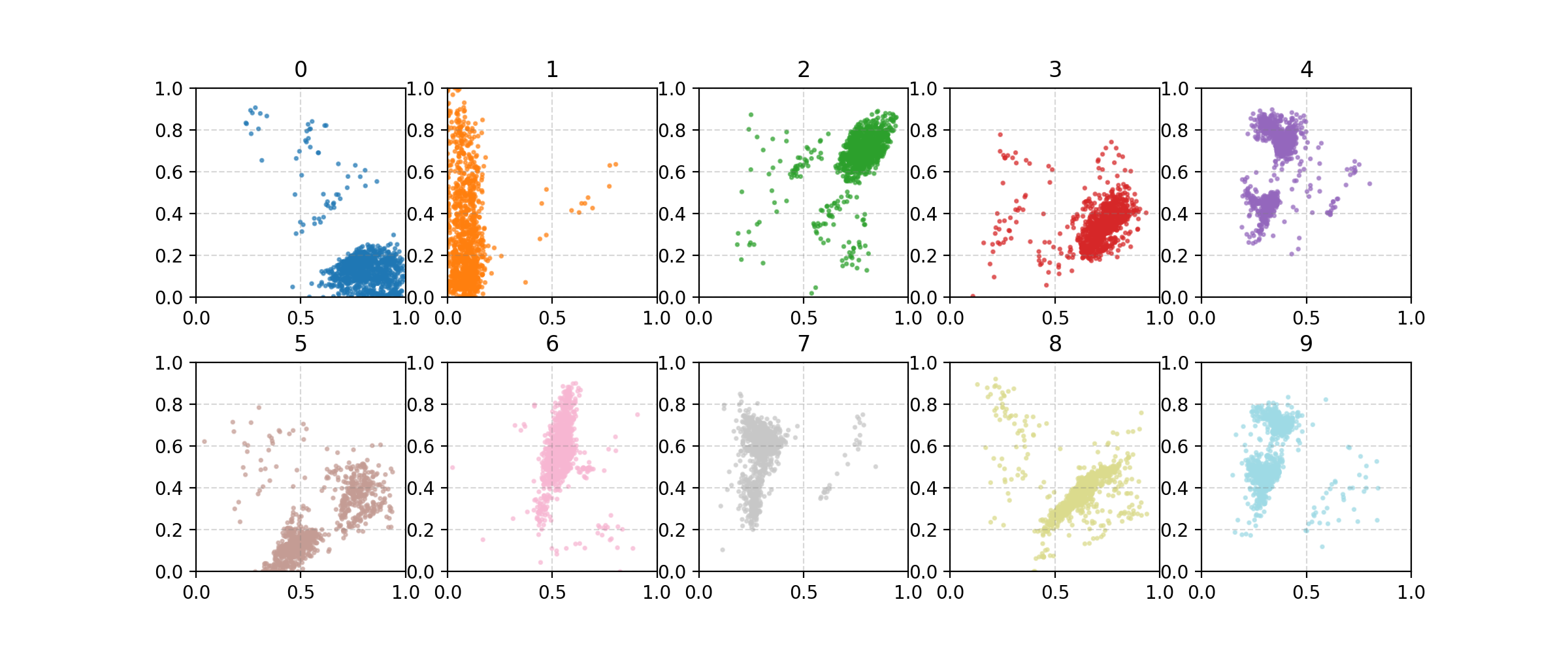
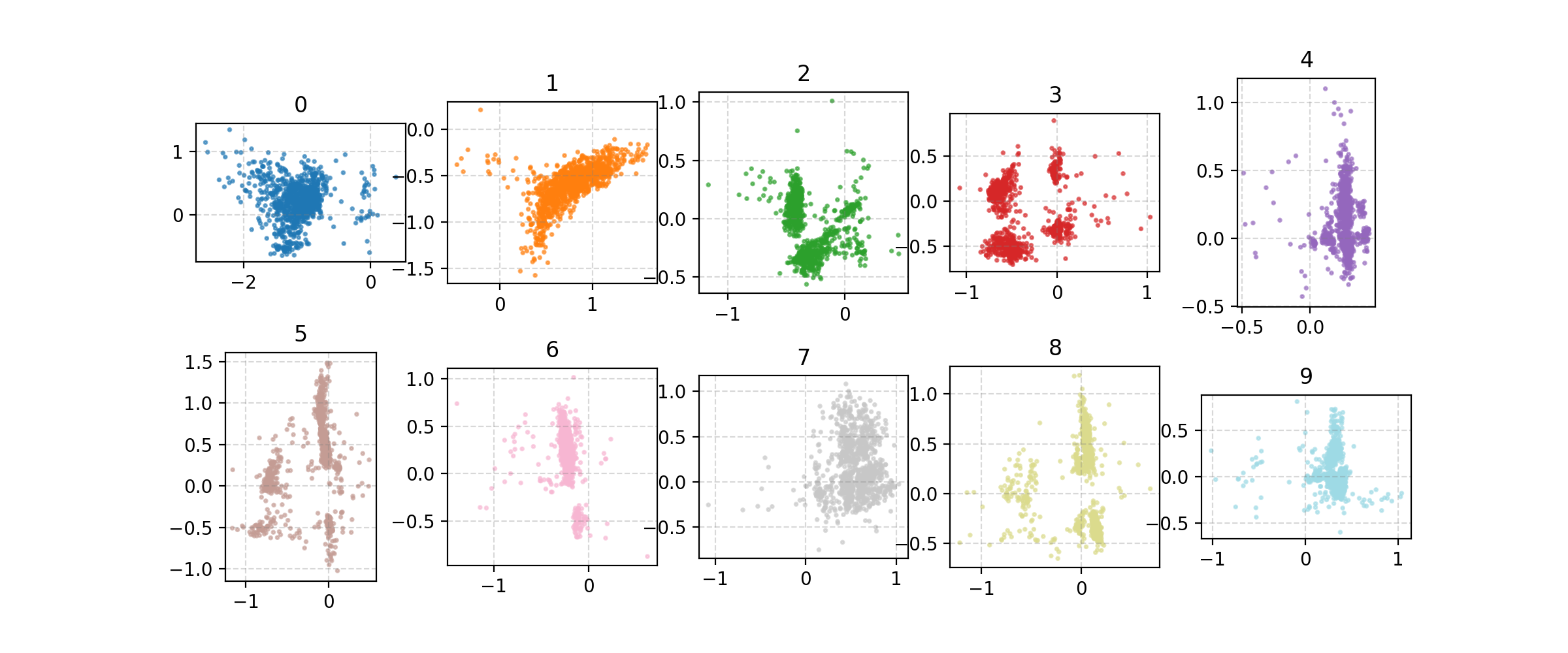
We can also look at where some of the test values are mapped into the latent space. It seems that the spherical VAE has the best separation which makes sense based on our reasons for constructing it.

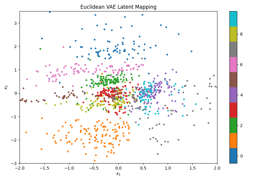
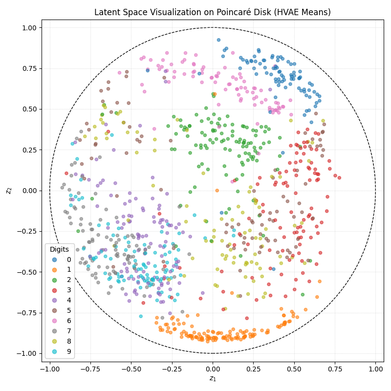
Of course the curved space latent spaces are just projections, we can do a little better if we embed them in a high dimensional Euclidean space (still projections but less compressed).
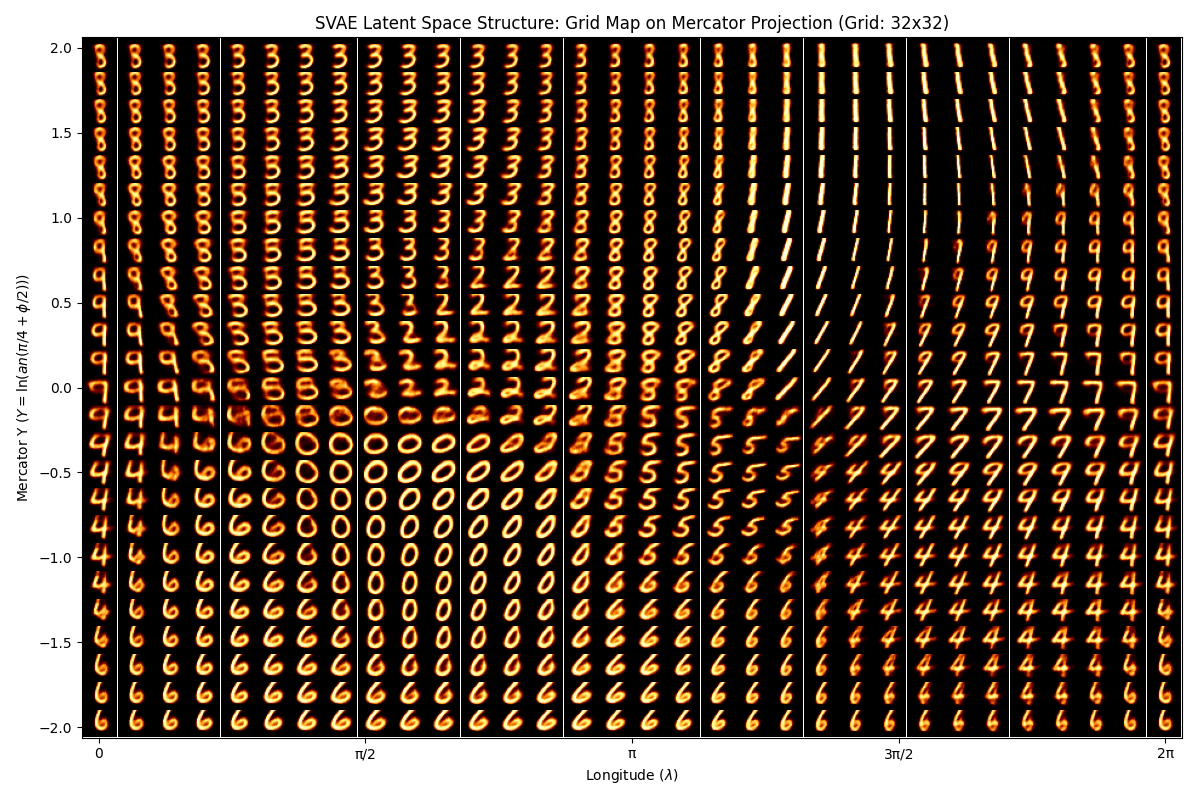
We can also observe how coordinates in the latent space map into as outputs.
— SVAE Latent Space —
— EVAE Latent Space —
— HVAE Latent Space —
What we’ll do from here is compare the negative log-likelihood or ELBO values for the different methods as a proxy for the evidence. This won’t be exact because the ELBO is a lower bound on the actual evidence where the difference is the KL divergence between the approximate and true distributions. But the ELBO is very easy to get with my current code so we’ll be using it regardless just to get a feel for the results are.
We’ll observe how well the different approaches do for varying latent dimensions, number of layers and number of nodes (the latter two basically to make sure our conclusions on the latent dimensions are more solid). Uncertainties are just derived from the variance of the loss on different batches of the testing dataset. And I should emphasize that this is not a proper report on the performance of these methods just a quick check that I did with lots of stuff that one would do better if they wanted rigorous results, so grain of salt and everything.
| Latent Dimensions | No. Hidden Layers | Euclidean VAE | Spherical VAE | Hyperbolic VAE |
|---|---|---|---|---|
| Dim = 2 | 1 | -170.8 +/- 9.9 | -168.9+/- 10.1 | -174.0 +/- 8.0 |
| 2 | -165.5 +/- 10.4 | -163.7 +/- 10.0 | -170.4 +/- 7.3 | |
| 3 | -166.8 +/- 10.8 | -160.2 +/- 9.8 | -171.5 +/- 7.3 | |
| Dim = 3 | 1 | -160.4 +/- 9.0 | -159.9 +/- 9.6 | -155.6 +/- 6.6 |
| 2 | -156.6 +/- 9.4 | -152.8 +/- 8.5 | 156.7 +/- 7.1 | |
| 3 | -154.4 +/- 9.3 | -154.7 +/- 9.3 | -155.8 +/- 6.7 | |
| Dim = 5 | 1 | -144.4 +/- 8.2 | -146.2 +/- 7.5 | -140.6+/- 5.5 |
| 2 | -140.7 +/- 7.8 | -145.2 +/- 7.4 | -139.2 +/- 6.1 | |
| 3 | -146.7 +/- 8.4 | -156.0 +/- 8.2 | -138.6 +/- 5.7 | |
| Dim = 10 | 1 | -130.7 +/- 5.9 | -141.4 +/- 6.9 | -123.4 +/- 4.7 |
| 2 | -134.0 +/- 6.6 | -145.6 +/- 6.8 | -122.0 +/- 4.4 | |
| 3 | -145.0 +/- 7.5 | -164.4 +/- 9.1 | -121.2 +/- 4.5 | |
| Dim = 50 | 1 | -131.9 +/- 6.4 | -195.5 +/- 11.1 | -163.1 +/- 6.6 |
| 2 | -138.4 +/- 6.6 | -201.2 +/- 11.6 | -205.1 +/- 10.5 | |
| 3 | -146.2 +/- 8.0 | -197.2 +/- 11.0 | -192.6 +/- 9.4 |
They do seem to roughly match up with what was reported in Nagano et al. (2019) and Davidson et al. (2018) at least in terms of the vanilla VAE outperforming the new methods in higher dimensions and the SVAE doing very well in low dimensions. Presumably because then the latent space has enough expressive power to kind of just do what I need to do, while the new methods of some instabilities that we had to introduce that may be coming out in higher dimensions but are more expressive in low dimensions as their structure matches the data.
The overall winner for the MNIST data seems to be the HVAE model with 10 latent dimensions (\(\mathbb{H}^{10}\)) with 3 hidden layers.
Labeled Faces in the Wild
The labelled faces in the wild dataset (kaggle/formal) is described as …
“Labeled Faces in the Wild (LFW) is an open source dataset aimed at researchers that was intended to establish a public benchmark for facial verification. Created by the University of Massachusetts, Amherst, and publicly released in 2007, LFW comprises over 13,000 facial images with different poses and expressions, under different lighting conditions. Each face is labeled with the name of the person, with 1,680 people having two or more distinct photos in the set.” - Labeled Faces in the Wild - dataset www.aiaaic.org
If we look at faces with more than 70 different images we over-sample different politicians.
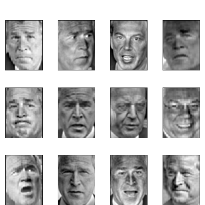
So we’ll quickly recap what we did in the last section. For a 2D dimensional latent space we can visualise how well each method reconstructs the data…. you ready for some nightmare fuel?
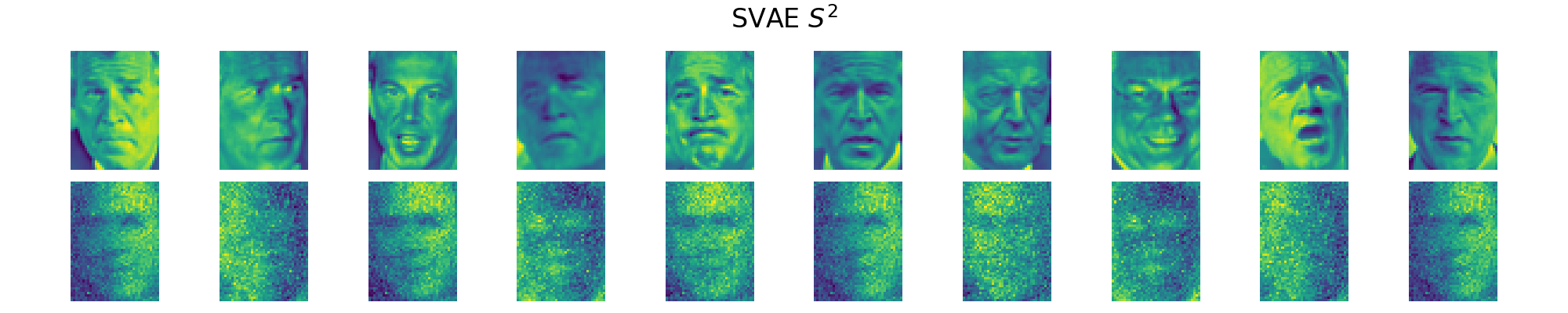
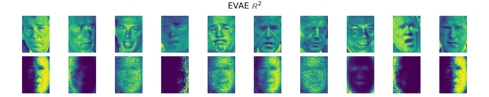
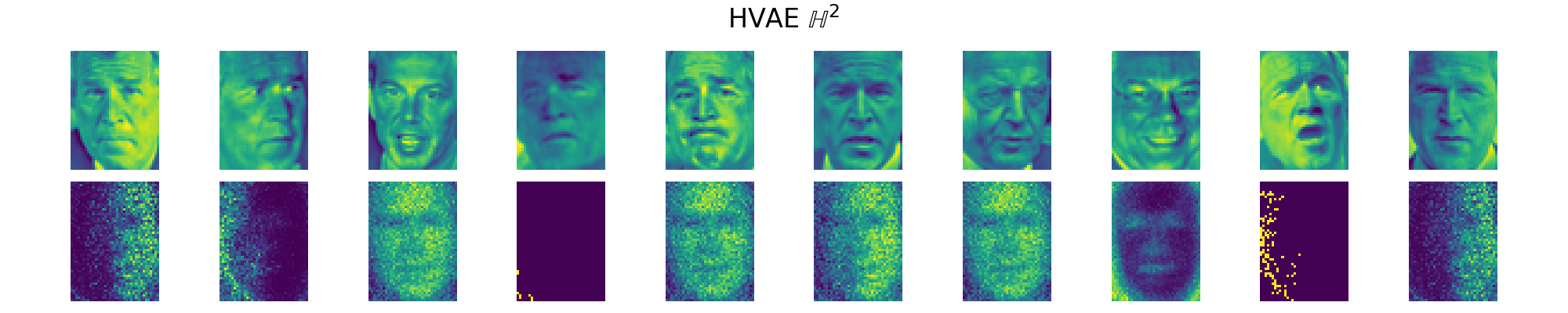
So … not great? But this is to be expected coz the data is slightly more complicated (sarcasm).
I’m not going to bother with showing how the latent space maps to the output as I could already tell that it would be uninterpretable, but we can at least look at how the inputs map to the latent space.
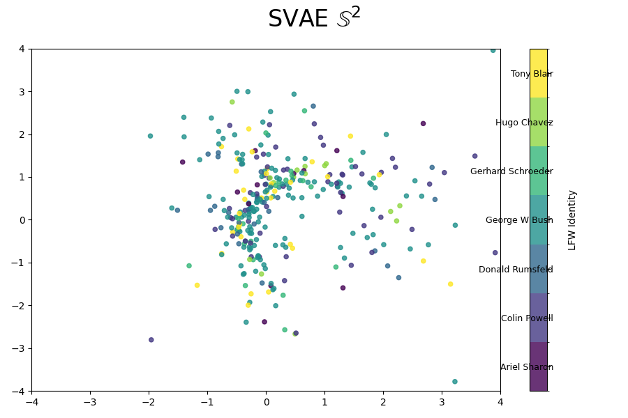

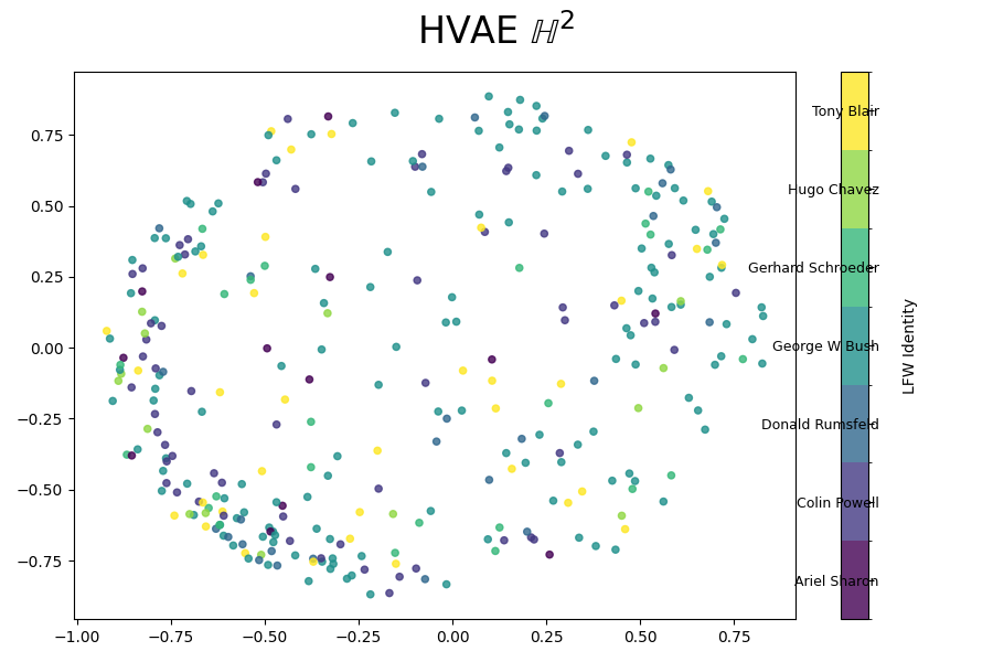
In which we can see that there is no rhyme or reason when it comes to who is who (yet).
Let’s look at some quantitative estimates for how well the different methods are reconstructing the images (however note the uncertainties…)
| \(D\) (Latent Dims) | \(L\) (Hidden Layers) | Euclidean VAE | Spherical VAE | Hyperbolic VAE |
|---|---|---|---|---|
| 2 | 1 | -975.2 +/- 66.0 | -1047.0 +/- 40.5 A2 | -1059.3 +/- 44.7 |
| 2 | -1065.0 +/- 40.4 | -1048.9 +/- 59.7 | -1041.8 +/- 47.1 | |
| 3 | -1017.5 +/- 62.0 | -1056.2 +/- 76.1 | -1020.2 +/- 42.5 | |
| 4 | -1009.1 +/- 64.7 | -1064.6+/- 50.5 | -1086.1 +/- 49.7 | |
| 3 | 1 | -966.9 +/- 57.1 | -1077.1 +/- 41.3 | -1004.6 +/- 51.7 |
| 2 | -1000.4 +/- 63.7 | -1067.4 +/- 52.5 | -1001.2 +/- 48.5 | |
| 3 | -1014.2 +/- 63.2 | -1068.4 +/- 59.6 | -1008.6+/- 51.4 | |
| 4 | -1020.2 +/- 61.0 | -1105.3 +/- 58.7 | -1006.1 +/- 47.7 | |
| 5 | 1 | -991.1 +/- 59.5 | -1136.4 +/- 35.9 | -987.0 +/- 55.6 |
| 2 | -1020.8 +/- 62.8 | -1054.8 +/- 61.4 | -1042.8 +/- 44.0 | |
| 3 | -1018.2 +/- 64.5 | -1099.9 +/- 40.6 | -991.45 +/- 60.8 | |
| 4 | -1017.7 +/- 68.4 | -1118.8 +/- 40.2 | -1014.7 +/- 44.1 | |
| 10 | 1 | -980.7 +/- 58.4 | -1133.7 +/- 36.6 | -1009.2 +/- 62.5 |
| 2 | -1032.6 +/- 62.9 | -1140.7 +/- 39.9 | -1022.7 +/- 66.0 | |
| 3 | -1025.3 +/- 67.9 | -1110.1 +/- 44.5 | -1008.4 +/- 59.9 | |
| 4 | -1026.8 +/- 70.8 | -1075.4 +/- 47.1 | -1018.3 +/- 54.0 | |
| 20 | 1 | -991.9 +/- 60.5 | -1141.3 +/- 37.5 | -1057.5+/- 61.2 |
| 2 | -1028.8 +/- 54.6 | -1137.8 +/- 43.6 | -1048.1 +/- 49.5 | |
| 3 | -1025.2 +/- 60.5 | -1130.3 +/- 42.3 | -1007.2 +/- 56.6 | |
| 4 | -1028.0 +/- 70.6 | -1136.8 +/- 41.9 | -1047.8 +/- 54.5 |
And I can confirm that the values for higher layers and latent dimensions are in fact bad. The loss plateaus and I’ve implemented several what I thought were intelligent things to do with the learning rate scheduler but that didn’t do anything…
Molecular Structure Reconstruction for QM9 dataset with constant curavture VAEs
The QM9 dataset is a dataset containing the structural information for ~130,000 molecules that is a pretty common benchmark for machine learning approaches to molecular property prediction.
In the words of PyTorch Geometric or PyG their page that has the QM9 data (which I use), the dataset is described as…
The QM9 dataset from the “MoleculeNet: A Benchmark for Molecular Machine Learning” paper, consisting of about 130,000 molecules with 19 regression targets. Each molecule includes complete spatial information for the single low energy conformation of the atoms in the molecule.
Here we are interested in seeing whether we can compress this data efficiently with the approaches above.
I thought it would be interesting, as I thought the inherent data had bits of spherical (angular) data and hierarchical (tree-like/compounding dependent) data. However, we believe the below results to be true (and in hindsight it should have been obvious), it seems one of the above clearly dominates when it comes to efficient compression.
Method
What we do is throw away the relatively simple overall quantum property data and focus in on the structure of the molecules. We looks at the positions of different combinations of the molecules, groups of three defining a plane, and extract the angular positions between these planes. These are called dihedral-angles and they can be used instead of bond angles, as far as I know. The gifs below are my attempt at showing how this works in the case of a cis- and trans- molecular configuration.
The below two gifs then show how the dihedral angle, the angle between planes, changes based on the position of the node/atom ‘D’ from two different perspectives (for same angle, I show the same structure) (this is for definitional purposes, many of the angles are not physical).
For our experiment on the QM9 dataset we encode the angles into x, y pairs of \((cos(\theta), \sin(\theta))\).
We feed these positions in, which we say fall inbetween \(-180^\circ\), and \(+180^\circ\) for a consistent convention. Theoretically, the discontinuity that occurs because of the cutoffs at the bounds should have been hard to learn…
We feed the list of pairs of \((cos(\theta), \sin(\theta))\) into the VAEs (i.e. feed in all the angles between triplets of molecules in a given molecule), compress this into the latent space, decode these values to get new estimates \((cos(\theta'), \sin(\theta'))\), then run a simple \(\arctan\) on the outputs to see if we get the right angles out!
The reconstruction loss (irrespective of the KL divergence/regularisation loss) is a simple cosine similarity value of the angular output.
Quick Disclaimer
For the below results I utilised Claude (the LLM) quite a bit to handle plotting, primarily so I didn’t have to: pick out the right angles and put them in the right axis, make sure the colours were consistent, figure out how to make a polar projection with matplotlib (although after I did this, turns out it was actually pretty simple), automating the process so I could re-run it all efficiently, etc.
Results
Below are some of the results of the training using mpl-drip for the colour scheme. First let’s look at the loss curves of the different methods to see whether we trained them enough.
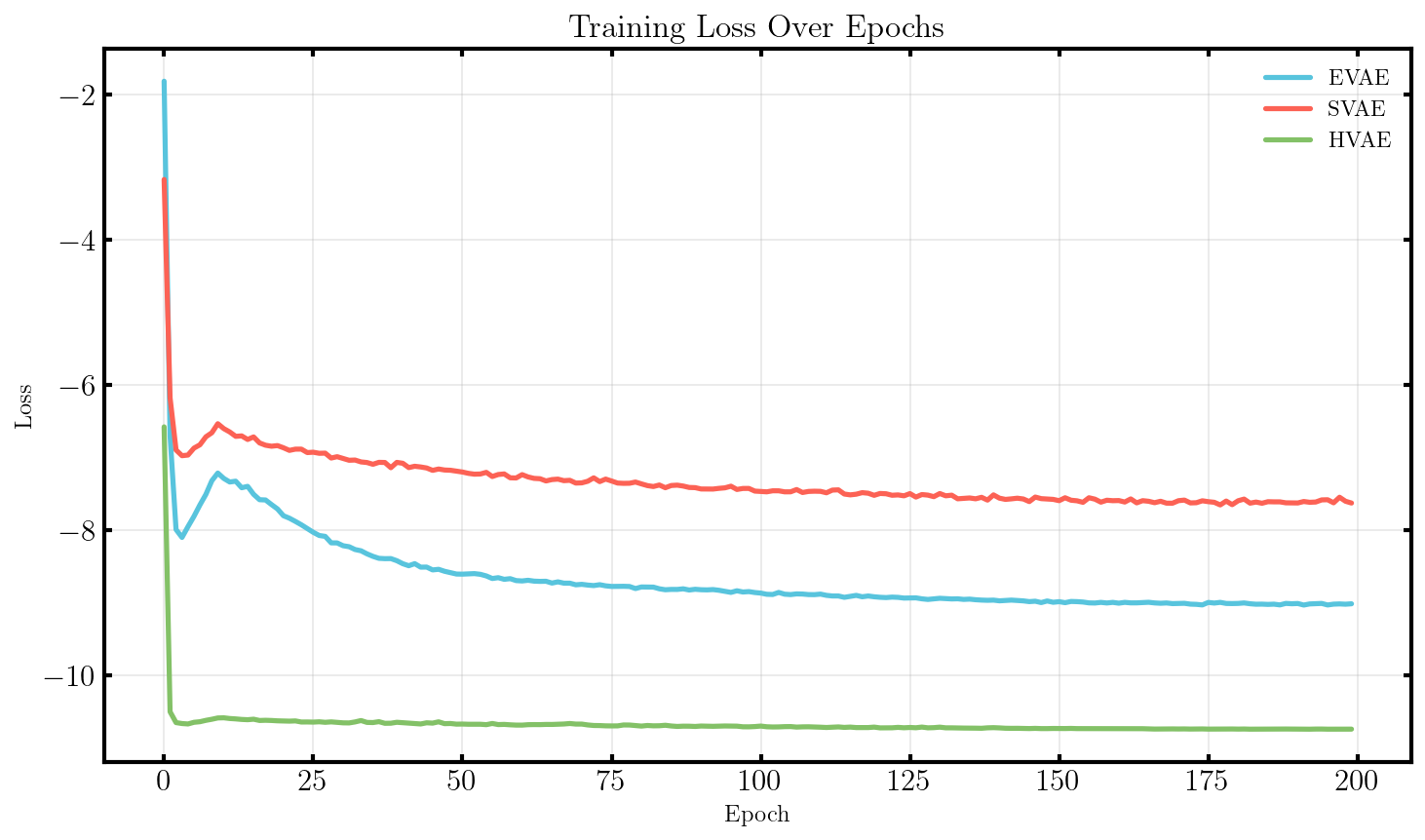
So right out of the gate, it seems that the HVAE (hyperbolic VAE) is getting something that the other VAE architectures don’t. Let’s see if that translates into performance though. Let’s look at the average angular error for the predictions, and the correlation of the angles with each other (if the VAE is picking up structure, we should find that the angles are related to each other –> higher correlations between the predictions).
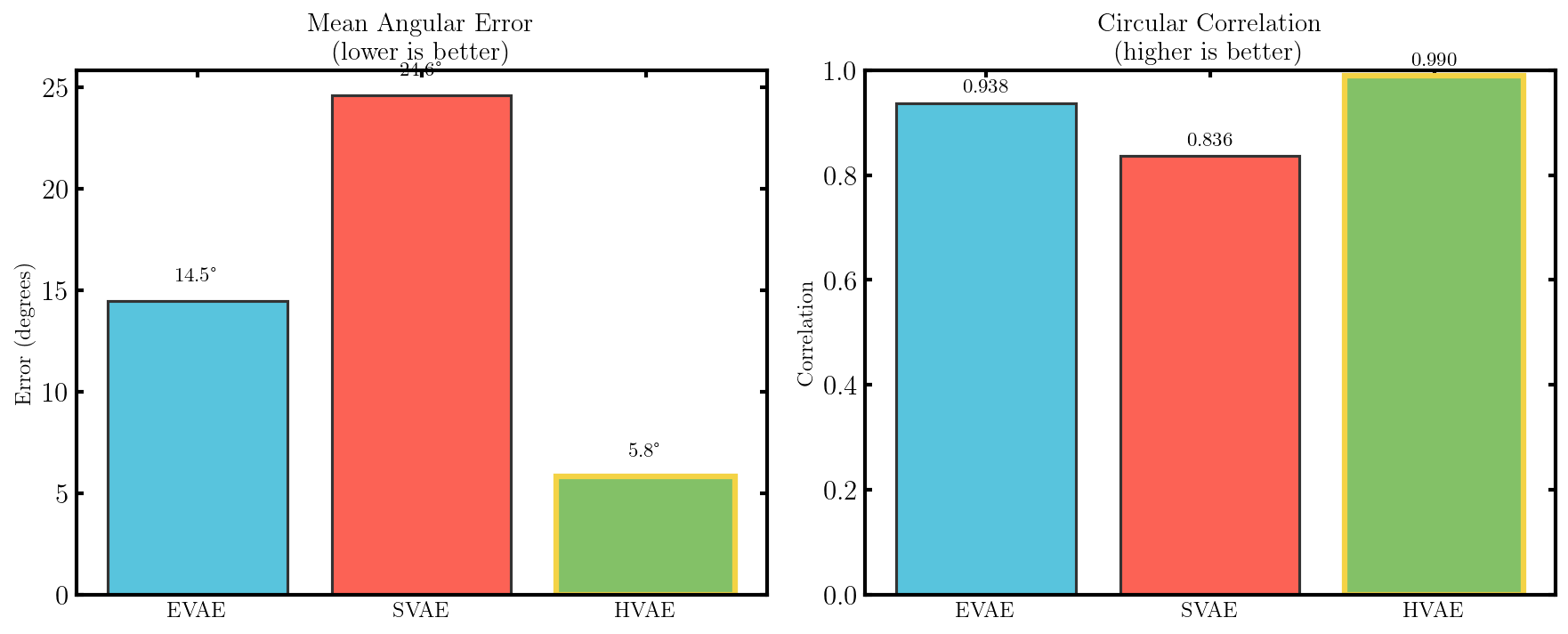
And while they do not do terrifically … the HVAE is still a clear winner. Looking at the overall results we find.
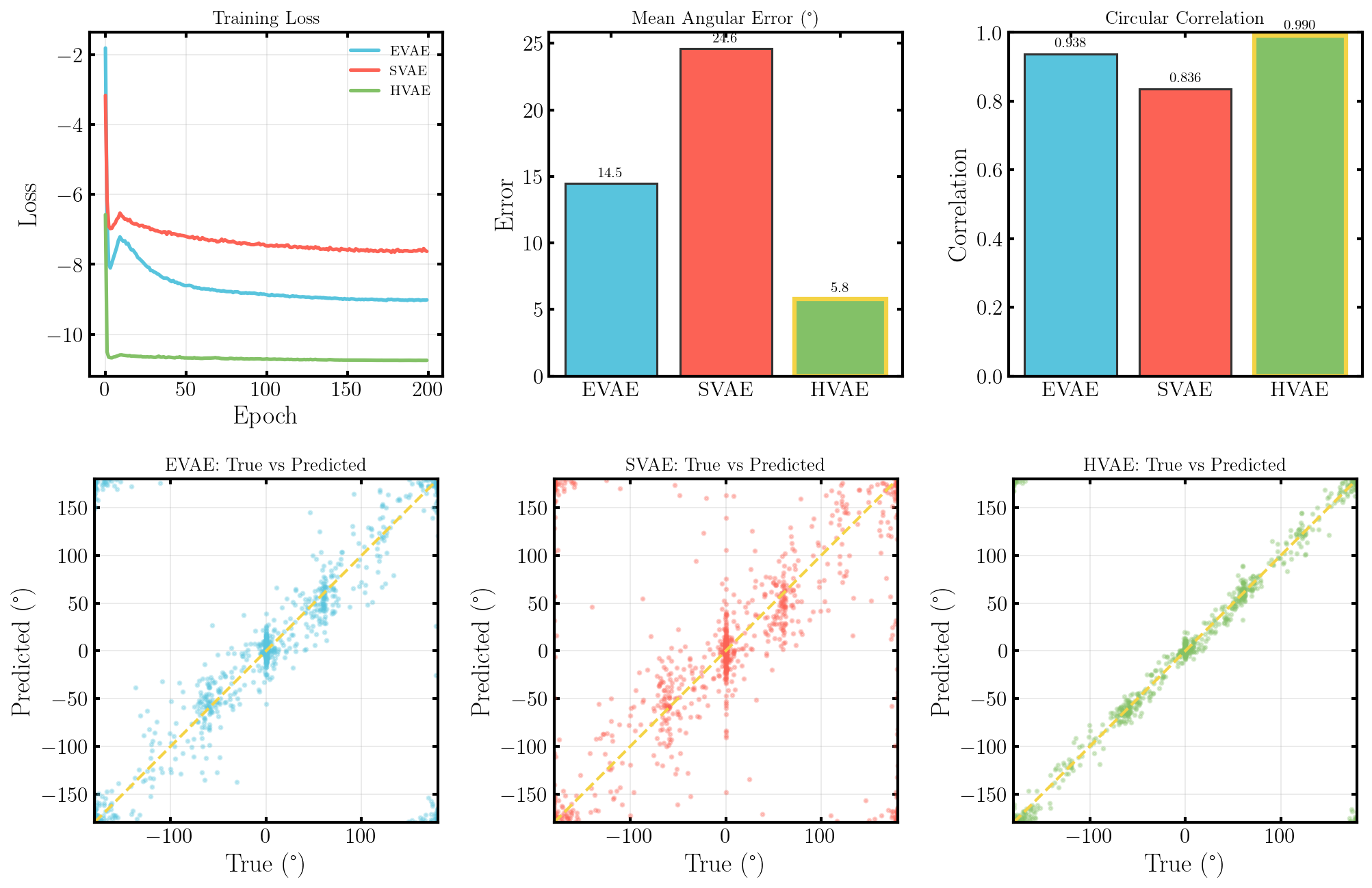
Looking a bit more at the distribution of errors, below I’ve made a plot that shows the angles on the unit circle for comparison (with some example connections to show true vs prediction) and the distribution of angular errors.

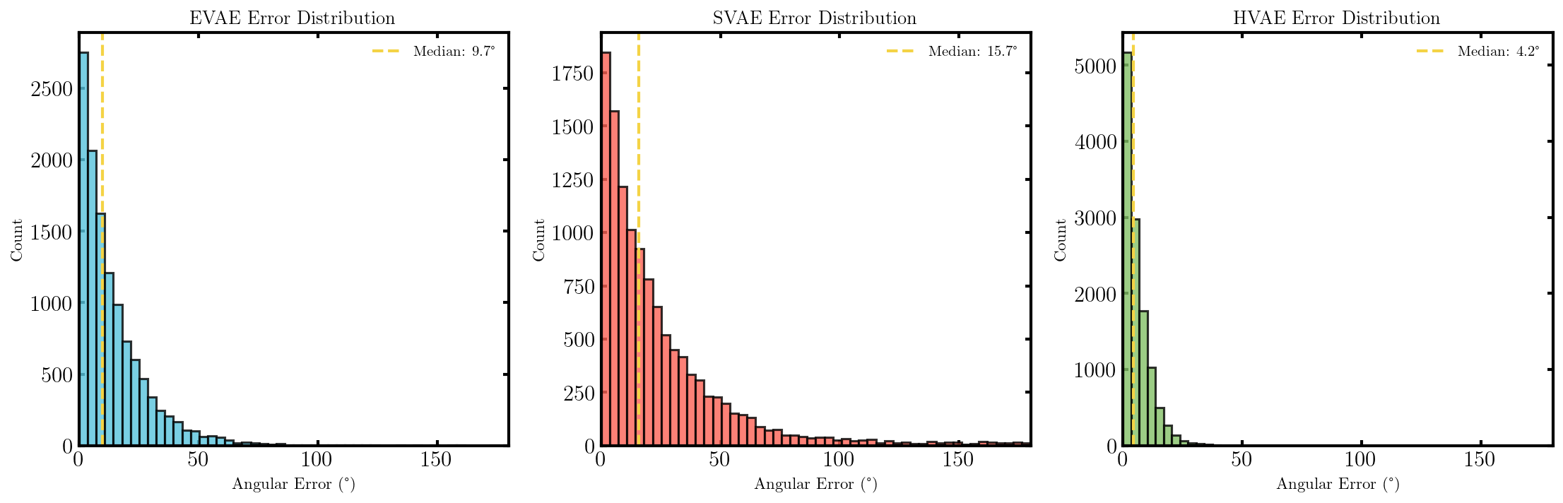
In which we can clearly see that the HVAE is picking up something that the EVAE and SVAE are not. Presumably this is because, as stated previously, the structure secretly has a lot of hierarchical structure because the molecule structures can be interpreted as very tree-like where the position of one angle depends on the previous and so on.
One extra thing that I thought might be happening is some imbalance in the set of target angles, so I used the best performing versions of the SVAE, EVAE and HVAE above and looked at there performances for specific ranges of angles. A particularly interesting region is ~-180 and ~+180, because theoretically the only network that can encode that these two values are exactly the same, would be the SVAE. However, in the above we can see a hint above that this behaviour isn’t captured by the SVAE any better than the other two methods.
Below we have some plots trying to show just that.
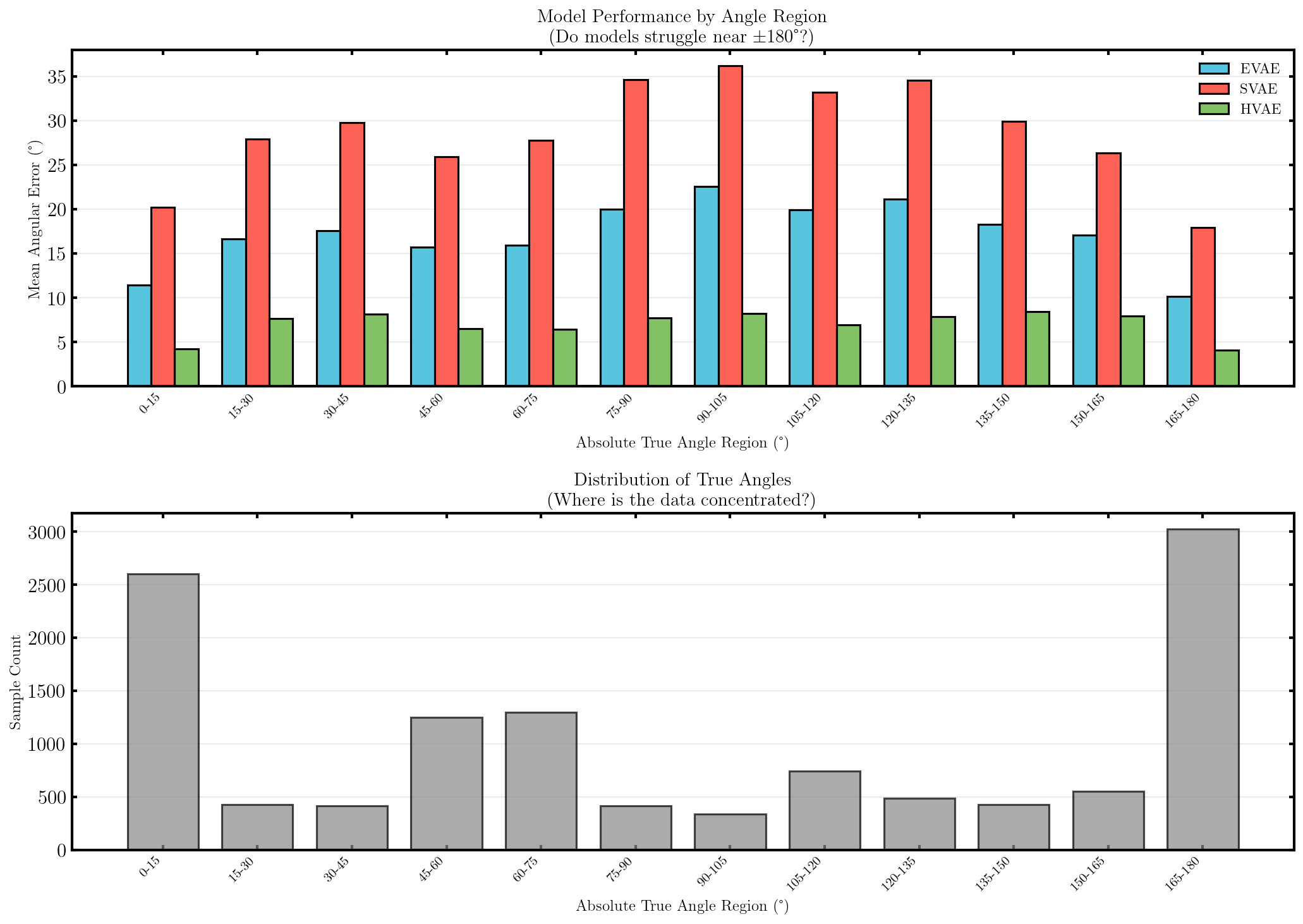
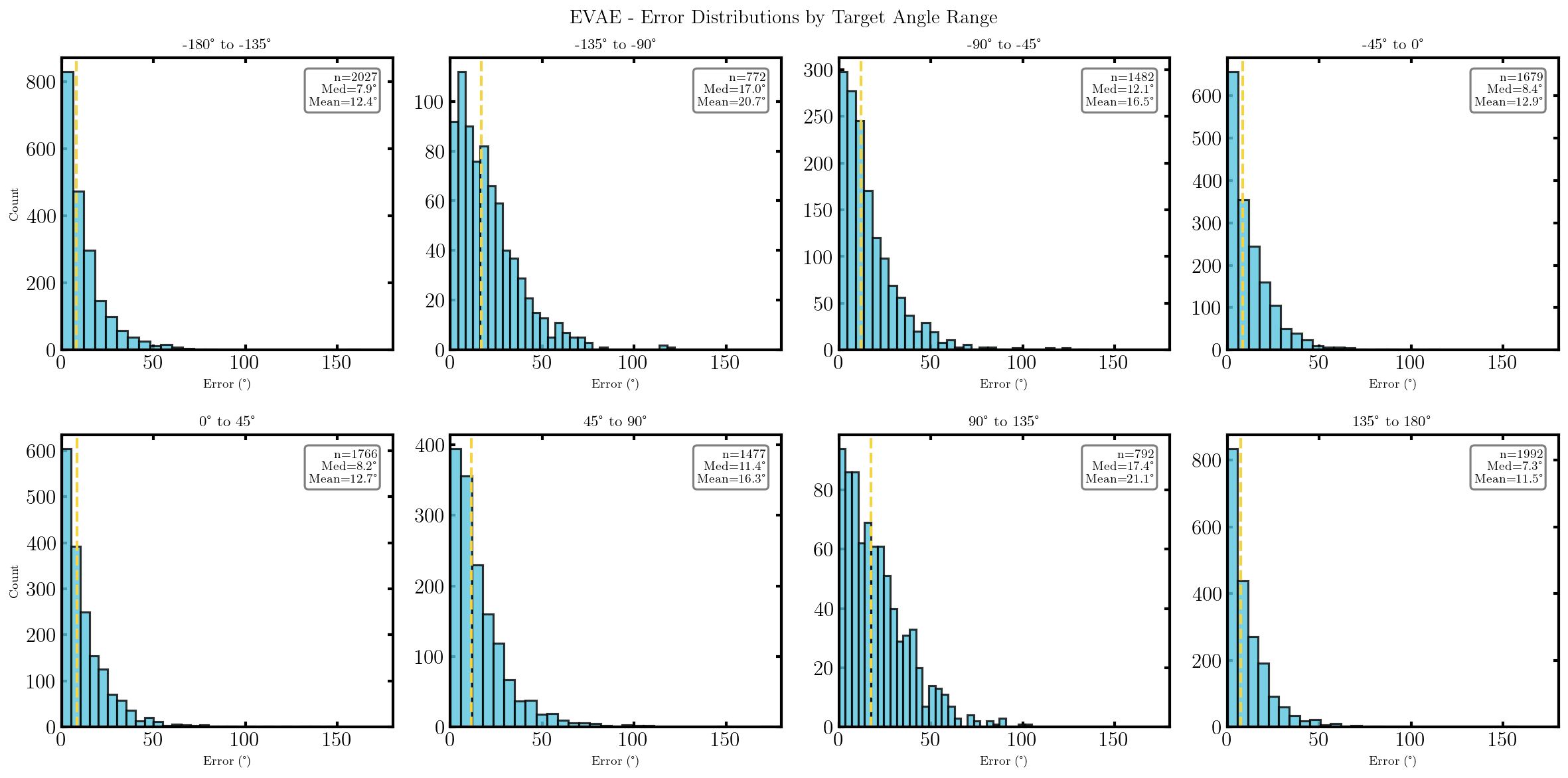
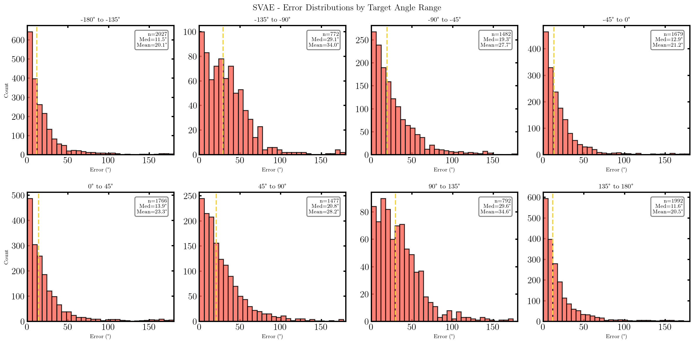
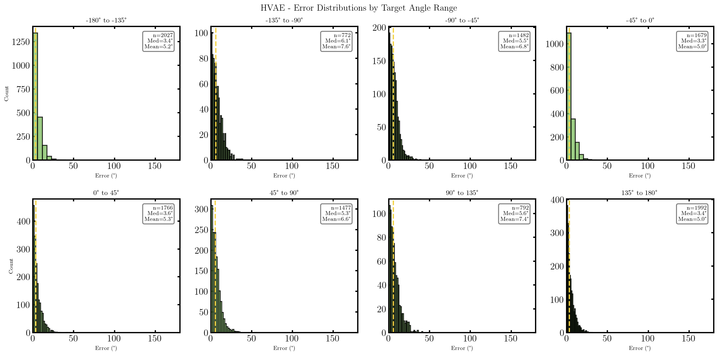
Basically it seems to come down to: less samples –> less accuracy.
Conclusions
Take everything I’ve presented here with a grain of salt, it’s just a blog post not a published article, it seems that there is utility in these methods at least, especially the HVAE to inherently hierarchical data it seems.
However, a major drawback to these methods is that it’s all or nothing. In the above QM9 experiment, it would make sense to have a bit of spherical and a bit of hyperbolic space, but by the constructions above the whole latent space has to be one or the other. This motivates the idea of Mixed-Curvature Autoencoders that alleviate this assumption/generalise the approach, that is on my list of ‘to do’s for these posts but we’ll see.
References
[1] Diederik P. Kingma, Max Welling. (2013). Auto-Encoding Variational Bayes. arXiv:1312.6114
[2] Diederik P. Kingma, Max Welling. (2019). An Introduction to Variational Autoencoders. arXiv:1906.02691
[3] Carl Doersch. (2016). Tutorial on Variational Autoencoders. arXiv:1606.05908
[4] Davidson, T. R., Falorsi, L., De Cao, N., Kipf, T., and Tomczak, J. M. (2018). Hyperspherical Variational Auto-Encoders. 34th Conference on Uncertainty in Artificial Intelligence (UAI-18). [GitHub Link]
Footnotes
Although it won’t be stylised and likely wouldn’t pass some basic standards for references but I don’t wanna do that by hand and markdown doesn’t exactly have a bibtex extension. ↩
The latent dimensional space of the VAE is presumed to have a lower dimension than the inputs. For the MNIST data (and images in general) it is presumed to be 1 dim per pixel or 784 total. Therefore the VAE compresses the data. ↩
You might think that the ‘centre’ for a unit sphere would just be the origin, but that point doesn’t lie on the sphere and so doesn’t exist within the spherical space. ↩
Notice that the loss only depends on \(\kappa\), not on \(\mu\). Meaning that \(\mu\) is only updated by the reconstruction loss. This makes a little sense as the value of \(\mu\) doesn’t really mean anything regularisation-wise. ↩
For the purpose of this post the usual notion of ‘curving’ is good enough. For a more general type of curvature that I usually default to thinking in terms of Gaussian curvature. ↩
I.E It exists within an N+1 dimensional Minkowski space. ↩
Not to be confused with the \(\kappa\) from the vMF distribution. ↩
If you’re wondering why the text is so close to the numbers it’s because the markdown file kept thinking that the numbering was restarting after each code block… ↩