
RJMCMC: What if you have an unknown number of parameters in your models? What if you don’t know which model is actually your model?
Published:
Heyo, in this post I’m going to describe how you can explore parameter spaces using MCMC in cases where you have a set of models with different numbers of parameters or more simply where you have a model with an unknown number of parameters using Reversible Jump Markov Chain Monte Carlo (RJMCMC). UNDER CONSTRUCTION
UNDER CONSTRUCTION UNDER CONSTRUCTION UNDER CONSTRUCTION UNDER CONSTRUCTION UNDER CONSTRUCTION UNDER CONSTRUCTION UNDER CONSTRUCTION UNDER CONSTRUCTION UNDER CONSTRUCTION UNDER CONSTRUCTION UNDER CONSTRUCTION UNDER CONSTRUCTION UNDER CONSTRUCTION UNDER CONSTRUCTION UNDER CONSTRUCTION UNDER CONSTRUCTION UNDER CONSTRUCTION UNDER CONSTRUCTION UNDER CONSTRUCTION UNDER CONSTRUCTION
Resources
- “Reversible Jump Markov Chain Monte Carlo Computation and Bayesian Model” - Peter Green (1995)
- “Advanced Simulation Methods || Chapter 7 - Reversible Jump MCMC” - Patrick Rebeschini (~2004 not sure)
- “Lecture 22. Reversible Jump MCMC” - N Zabaras, University of Notre Dame (2017)
- “Reversible jump Markov chain Monte Carlo and multi-model samplers” - Fan, Sisson and Davies (v1 2010/ v2 2024), arXiv:1001.2055v2
- “Efficient Construction of Reversible Jump Markov Chain Monte Carlo Proposal Distributions” - S. P. Brooks, P. Giudici, G. O. Roberts
- For various RJMCMC proposal methods
- “Model Choice using Reversible Jump Markov Chain Monte Carlo” - David Hastie, Peter Green (2011)
- “What are order statistics? - Equitable Equations (YouTube Video)
- “Towards Automatic Reversible Jump Markov Chain Monte Carlo” - David Hastie (PhD Thesis)
Table of Contents
- Statement of the problem
- Describing the mathematics of jumping between different dimensional spaces
- Examples
- Conclusion
Statement of the problem
It is quite common that when performing inference, a statistician doesn’t know a priori how many parameters they need to describe her data or which one of a collection of models actually describes the data. This falls outside the typical region in which general sampling techniques (such as MCMC), apply and thus requires some specialised treatment in the form of ‘trans-dimensional probability theory’ and ‘reversible-jump MCMC’.
Describing the mathematics of jumping between different dimensional spaces
Following a similar introduction but Fan et al. (2024), let’s say we have a set of data \(\mathcal{D}\) that comes from some model within a finite set of models \(\{\mathcal{M}_1, \mathcal{M}_2, \mathcal{M}_3, \dots, \mathcal{M}_k, \dots\}\) with \(k \in \mathcal{K}\) being used to indicate which model is currently being investigated and can be thought of as a new variable. Each model then has an \(n_k\)-dimensional set of parameters \(\theta_k \in \mathbb{R}^{n_k}\), where it’s not necessarily true that \(n_k = n_{k'}\).
Treating the variable \(k\) as an indicator for the (discrete) model distribution, the probability of a given model \(\mathcal{M}_k\) and its set of parameters \(\theta_k\) given the data \(\mathcal{D}\) is,
\[\begin{align} \pi(k, \theta_k \vert \mathcal{D}) = \frac{\mathcal{L}(\mathcal{D}|k, \theta_k) p(\theta_k, k)}{\sum_{k' \in \mathcal{K}} \int \mathcal{L}(\mathcal{D}|k', \theta_{k'}) p(\theta_{k'}, k') d\theta_{k'}} = \frac{\mathcal{L}(\mathcal{D}|k, \theta_k) p(\theta_k \vert k) p(k)}{\sum_{k' \in \mathcal{K}} \int \mathcal{L}(\mathcal{D}|k', \theta_{k'}) p(\theta_{k'}\vert k')p(k') d\theta_{k'}}. \end{align}\]Where the second equality is expanding \(p(\theta_k, k)\) to \(p(\theta_k \vert k) p(k)\), which is typically easier to encode. In essence, \(p(\theta_k \vert k)\) is just the prior on the set of parameters for the given model \(\mathcal{M}_k\), and \(p(k)\) is your prior or set of assumptions on which models describe your data a priori.
Presuming that we can nicely encode all this, next we want to know how to sample this posterior. Typical MCMC algorithms need to satisfy a detailed balance condition1 encoded by,
\[\begin{align} \int_{(\theta, \theta')\in \mathcal{A}\times\mathcal{B}} \pi(d\theta) P(\theta, d\theta') = \int_{(\theta, \theta')\in \mathcal{A}\times\mathcal{B}} \pi(d\theta') P(\theta', d\theta), \end{align}\]which says that assuming you’re generating samples of the distribution of interest then the probability of transitioning or the flow of probability, with \(P\) denoting the Markov transition kernel, between any two areas is proportionate to the probability mass in those regions. i.e. During sampling we don’t get more samples entering a region than the number leaving.
We then separate the kernel into a proposal distribution \(q\), which is whatever distribution you want but typically it’s a gaussian, and acceptance probability \(\alpha\) given by,
\[\begin{align} \alpha(\theta, \theta') = \min\left\{1, \frac{\pi(\theta' | \mathcal{D}) q(\theta', \theta)}{\pi(\theta | \mathcal{D}) q(\theta, \theta')} \right\}, \end{align}\]such that detailed balance is satisfied,
\[\begin{align} \int_{(\theta, \theta')\in \mathcal{A}\times\mathcal{B}} \pi(d\theta) \alpha(\theta, \theta') q(\theta, d\theta') = \int_{(\theta, \theta')\in \mathcal{A}\times\mathcal{B}} \pi(d\theta') \alpha(\theta', \theta) q(\theta', d\theta). \end{align}\]The math for RJMCMC is then just substituting \(\theta = (k, \theta_k)\) and \(\theta' = (k', \theta_{k'}')\) plus accounting for the transformations’ jacobians. To simplify things, we then separate out the proposals and acceptance functions into two kernels or moves: a ‘within-model’ move, and a ‘between-model’ move.
The ‘within-model’ move is where we keep \(k\) fixed and do a standard MCMC move.
The ‘between-model’ move is where when jump in model space / stochastically sample \(k\) or jump between models (hence the name) and we deterministically transform \(\theta_k\) based on the jump. The between-model model acceptance probability for some arbitrary proposal is given by:
\[\begin{align} \alpha[(\theta_k, k), (\theta_{k'}', k')] = \min\left\{1, \frac{p(\theta_{k'}', k' | \mathcal{D}) q(k'\rightarrow k) q_{d_{k'} \rightarrow d_k}(u_{k'})}{p(\theta_{k}, k | \mathcal{D}) q(k\rightarrow k') q_{d_{k} \rightarrow d_{k'}}(u_k)} \left\vert \frac{\partial g_{k\rightarrow k'}(\theta_k, u_k)}{\partial (\theta_k, u_k)} \right\vert\right\}. \end{align}\]There are a few new pieces in this equation that are worth mentioning:
- \(q(k'\rightarrow k)\) represents the proposal distribution for between model jumps i.e. if I’m at model \(k'\) what is the probability that I will jump to model \(k\)?
- \(\theta_{k'}' = g_{k\rightarrow k'}(\theta_k, u_k)\) is the mapping of how we take the last sample \(\theta_k\) and \(u_k\) in model \(k\) to the parameter \(\theta_{k'}\) in model \(k'\).
- \(\frac{\partial g_{k\rightarrow k'}(\theta_k, u_k)}{\partial (\theta_k, u_k)}\) is the jacobian of the transformation of the parameters from model \(k\) to model \(k'\).
- \(u_k\) and \(u_{k'}\) are dummy parameter that are used when we move from model \(k\) to model \(k'\) to keep the size of the total parameter space constant. There are two main reasons for this:
- Computers do not like dealing with objects of different sizes during compilation, so to make the inputs and outputs the same size we add padding or ‘dummy’ dimensions to keep the sizes constant.
- To calculate a valid Jacobian determinant, the mapping \(g\) must be a diffeomorphism between spaces of matched dimensions (\(n_k + \dim(u_k) = n_{k'} + \dim(u_{k'})\)). Or more simply, to have a well defined jacobian we need the parameter space between any two models to be the same, but not necessarily the same across a whole run.
e.g. If model 1 has three parameters \(\{\theta_1^{(1)}, \theta_1^{(2)}, \theta_1^{(3)}\}\), and model 2 has 7 parameters \(\{\theta_2^{(1)}, \theta_2^{(2)}, ..., \theta_2^{(7)}\}\) and we know that the max size of parameter space for the models is 10. Then, for model 1 we add a 7 parameter vector \(\vec{u}_1\) that doesn’t contribute to the prior or likelihoods (except it’s own prior which is next) and for model 2 we add a 3 parameter vector \(\vec{u}_2\) so that the inputs and outputs of the parameter space are both size 10.
- i.e. \((\theta_{k'}, u_{k'}) = g_{k\rightarrow k'}(\theta_k, u_k)\) and \(\textrm{dim}(\theta_k) + \textrm{dim}(u_k) = \textrm{dim}(\theta_{k'}) + \textrm{dim}(u_{k'})\)
- \(q_{d_{k} \rightarrow d_{k'}}(u_{k'})\) is the density that we generate \(u_{k'}\) from given that we started at \(k\), typically the density is taken to be unconditional, independent and uniform in each dimension of \(u_{k'}\) e.g. If \(u_{k'}\) is three dimensional then \(q_{d_{k'}}(u_{k'})= \prod_{i=1}^3 \otimes \mathcal{U}(u_{k'}^i)\).
In next few couple sections I’ll go into specific examples to further clarify some stuff relating to choices for \(q(k'\rightarrow k)\), \(g_{k\rightarrow k'}\), \(u_k\), and \(q_{d_{k} \rightarrow d_{k'}}(u_{k'})\).
Critically, the design of \(g\), \(q_k\), and \(u_k\) for a problem so that acceptance is non-negligible is the hardest part in all of this. In the next few sections I’ll go through some possibilities for \(g\) in particular, with a few examples showing example \(q_k\) and \(u\). In no way is it exhaustive, but it should hopefully give you an idea.
Methods to Combat Identifiability Issues
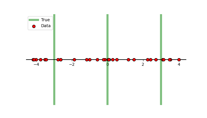
Before jumping (see what I did there) into the different types of proposals I feel that it would be non-representative … not practical … bad, to not go through methods to combat identifiability issues. These methods basically impose structure on the parameters such that we eliminate issues where a posterior has a bunch of modes and symmetries because multiple components look exactly the same and can represent the same features in the data. This identifiability issues happens very often trans-dimensional models but is not restricted to them. For example, let’s say that we have some 1D data that we know comes from 3 normals with known equal width and amplitude, but we don’t know their positions.
In a typical setup, our prior on the positions would be uniform,
\[\pi(\vec{\mu})= \begin{cases} C & \textrm{if }\vec{\mu}\in [-5, 5]^3\\ 0 & \textrm{else}\end{cases},\](putting additional bounds to make some ease-of-use). The likelihood for our data \(x\) would then be,
\[\begin{align} \mathcal{L}(x \vert \vec{\mu}) = \sum_{i=1}^3 \frac{1}{3} \mathcal{N}(x \vert \mu_i, \sigma^2 = 1). \end{align}\]We’ll set the true values of the gaussians to be \(-3\), \(0\) and \(+3\) to generate our data.
Now instead of running MCMC or performing variational inference, we’re going to do what we would usually label as the ‘dumb thing’ and brute force scan the parameter space to see what our posterior looks like. The result is in the same style as a corner plot where we are looking at the marginals of the posterior.
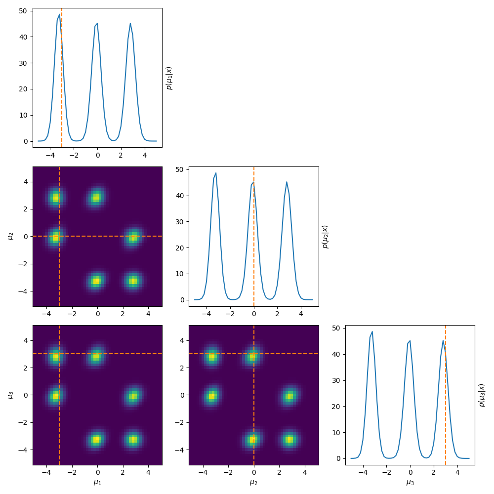
To put it in very esoteric and technical language … this bad. This very bad.
As stated above, this is an extremely common problem in trans-dimensional problems where added components are non-identifiable and samplers often have issues of label-switching. But in general it just means that the posterior is multi-modal, which is pretty much always harder to converge on.
To combat this we enforce structure on the posterior by either reducing or excluding the possibility of label switching, and in general these methods fall under the umbrella of order statistics (heads up that the link is a video) which is generally broader than what I’m using for here and literally relates to the statistics about the ordering of parameters. I’m not going to go very deep into the math here and instead simply focus on what the relevant posteriors look like and make conclusions on that2.
The first thing we’re going to try is simply mask regions that we don’t like. If we want \(\mu_1 < \mu_2 < \mu_3\), then when this isn’t satisfied we just set the probability to zero. The python prior and likelihood for this would look like the below (optimised to take in a vector of each parameter at once where the first dimension denotes which parameter).
def log_prior_mask(mu):

    log_prior = stats.uniform(*prior_bounds).logpdf(mu)

    log_prior = np.where(mu[0]>mu[1], -np.inf, log_prior)
    log_prior = np.where(mu[1]>mu[2], -np.inf, log_prior)
    log_prior = np.where(mu[0]>mu[2], -np.inf, log_prior)

    return log_prior.sum(axis=0)

def individual_log_likelihood(x, mu):
    log_weights = np.log(weights)
    log_pdfs = [log_weights[i] + stats.norm(loc=mu[i], scale=scale).logpdf(x) for i in range(len(mu))]

    return special.logsumexp(log_pdfs, axis=0)
This prior produces the following posterior.
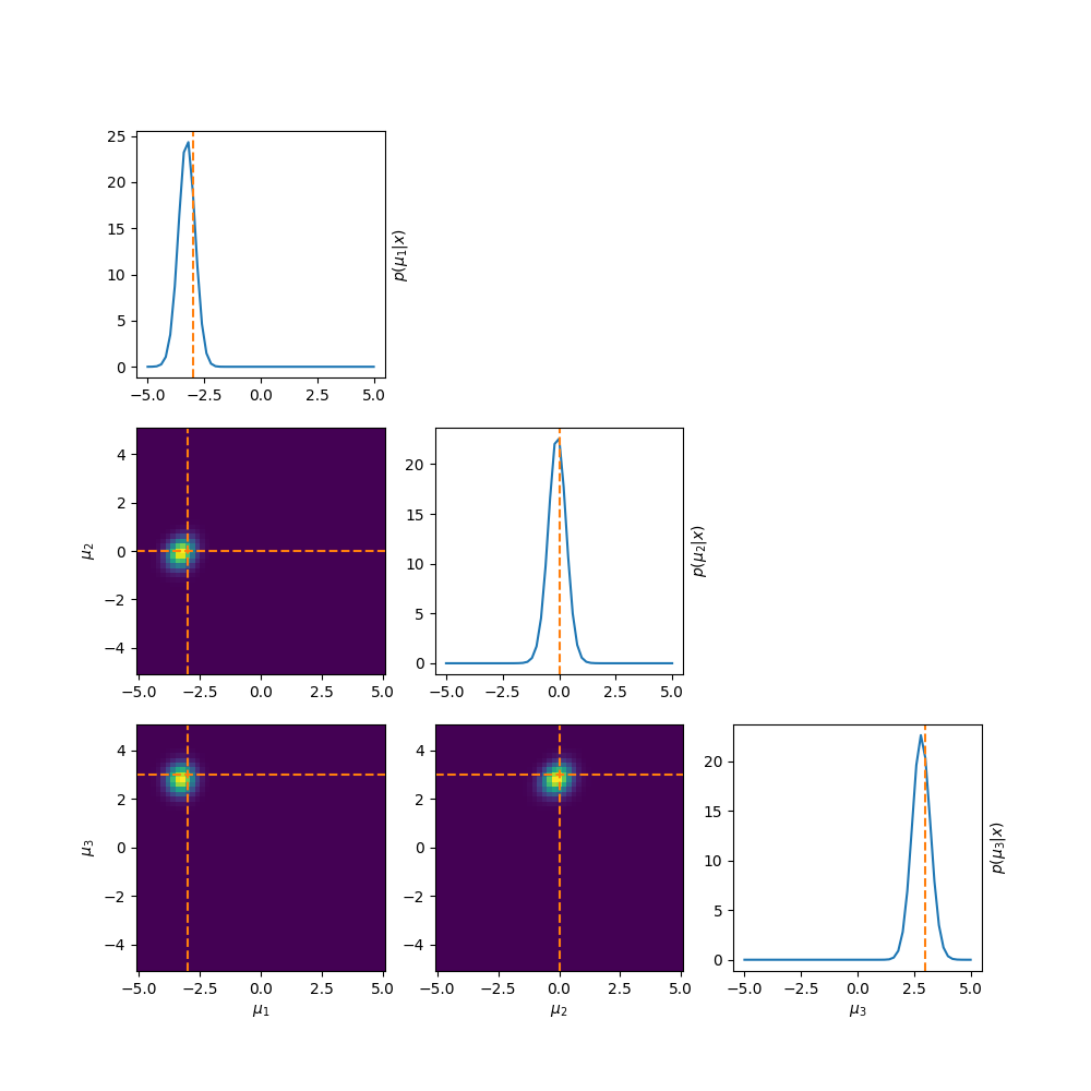
Which by eye doesn’t look too bad right, at least it’s better than before. But if we look at the log-posterior instead we can see one big issue.
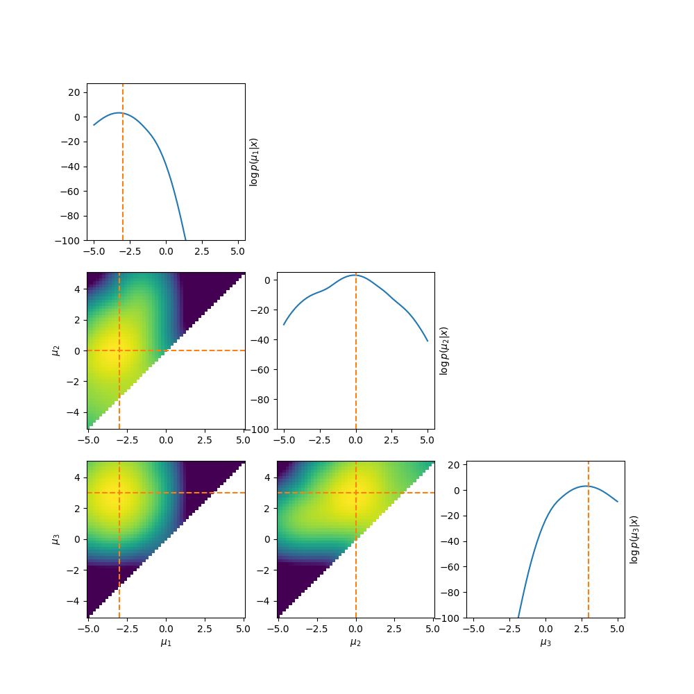
The abrupt cutoff can cause a lot of issues with samplers3. This motivates us to think of other ways to enforce the ordering.
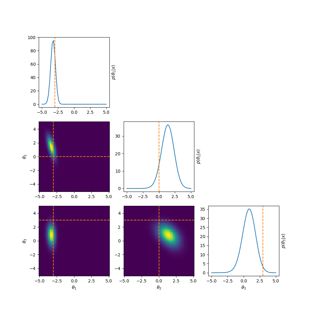
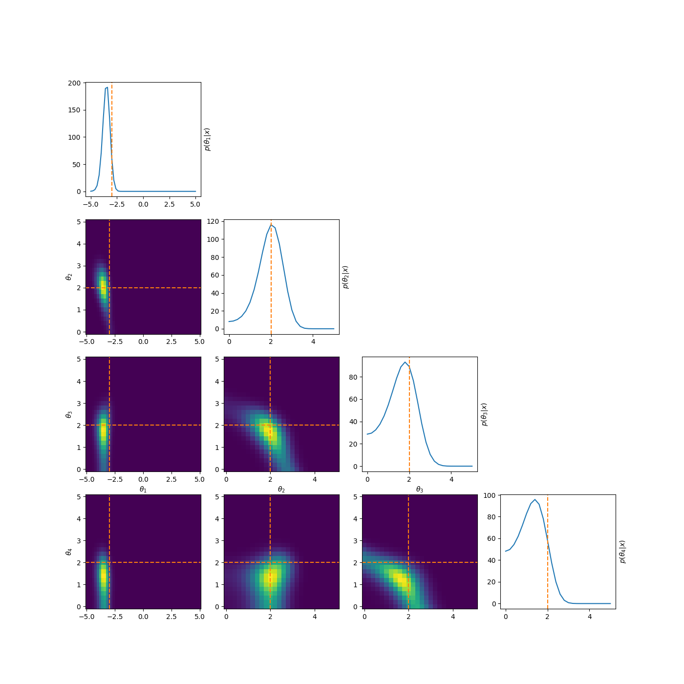
One example of this that’s a little more involved, is to reparamterise the problem to look at analysing the differences between the parameters. i.e. If we have \((\mu_1, \mu_2, \mu_3)\) then instead we look at \((\theta_1, \theta_2, \theta_3) = (\mu_1, \mu_2-\mu_1, \mu_3-\mu_2)\). This introduces correlations and non-gaussian behaviour but doesn’t have the abrupt cutoff. And as for the correlations, I have some example posteriors in the case of 3, 4, 5 and 6 component mixtures.
This can also be done to order the components based on amplitude or SNR when that distinguishes the components such as in astrophysical signals in astrometry or gravitational wave analysis.
Similarly, let’s say we want the means to be constrained within the \((-5,5)\) range that would be a little hard above as the uniform distribution that I’m evaluating the differences of would be a function of the previous parameters. One way to more easily do this is via a stick-breaking or Dirichlet process.
The ‘stick-breaking’ nature of the process is in relation to the parameters kind of like being the broken parts of a stick being broken, such that when added together one recovers the stick. You can see this in the very sophisticated diagram below that I definitely didn’t just make in powerpoint.
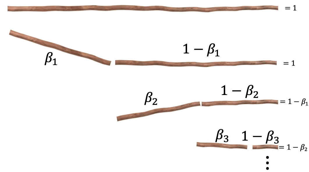
Where \(\vec{\beta}\) are now the parameters of interest that satisfy \((1-\beta_1) + \beta_1 = 1\) and \((1-\beta_2) + \beta_2 = 1\) and \((1-\beta_3) + \beta_3 = 1\) and so on such that fractions of the stick add up back to the original, or \(1 = \beta_1 + (1-\beta_1)\cdot(\beta_2 + (1-\beta_2)\cdot ((1-\beta_3) + \beta_3 ))\). In our case though, instead of it being a interval of length 1 starting at 1, it’s our \((-5, 5)\) interval, where ‘breaks’ are the positions of our normal distributions. This also enforces that the next mean/centre has to be to the right of the previous.
I won’t go through the math in much detail4, but basically we define the $\vec{\beta}$ up to some jacobian shananigans by,
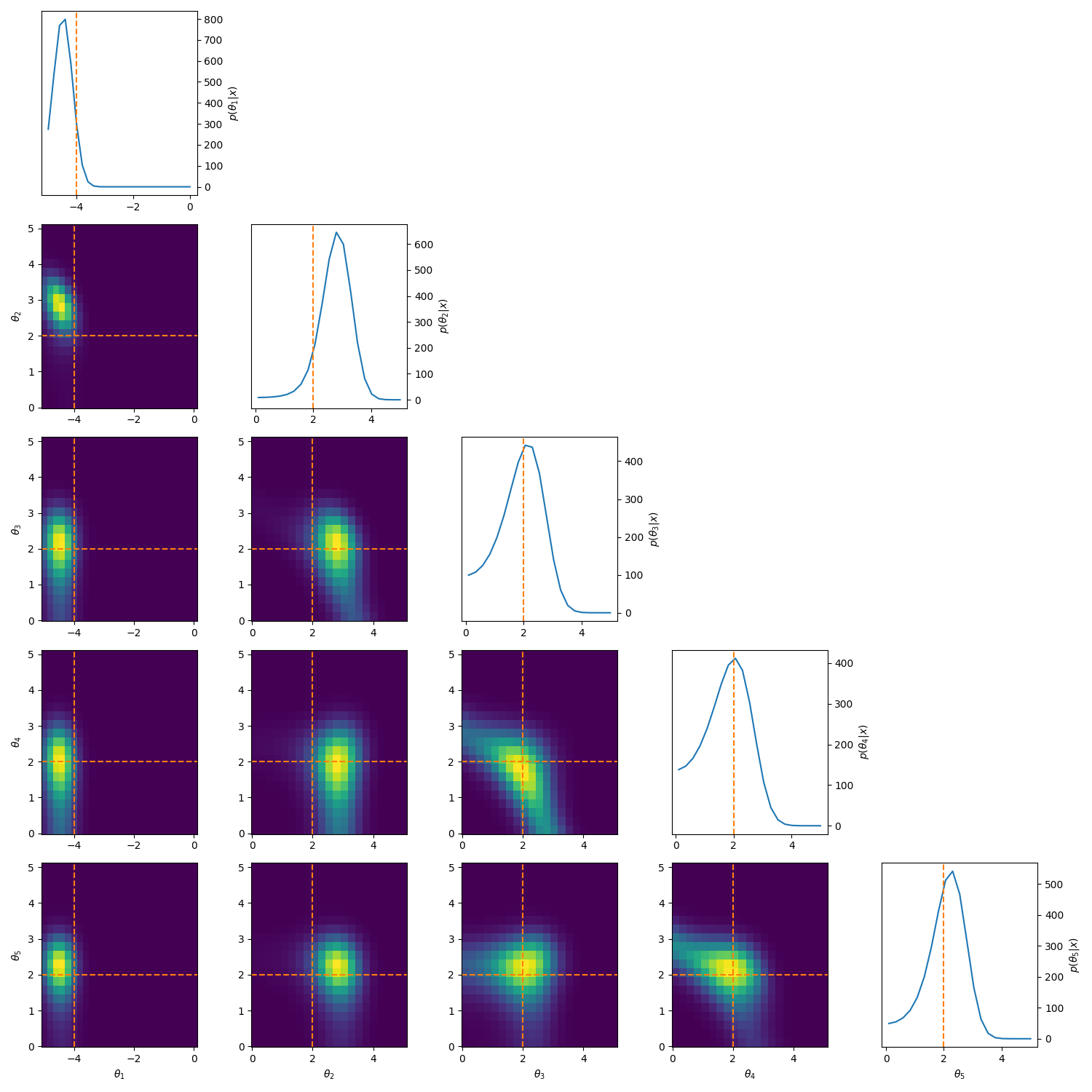
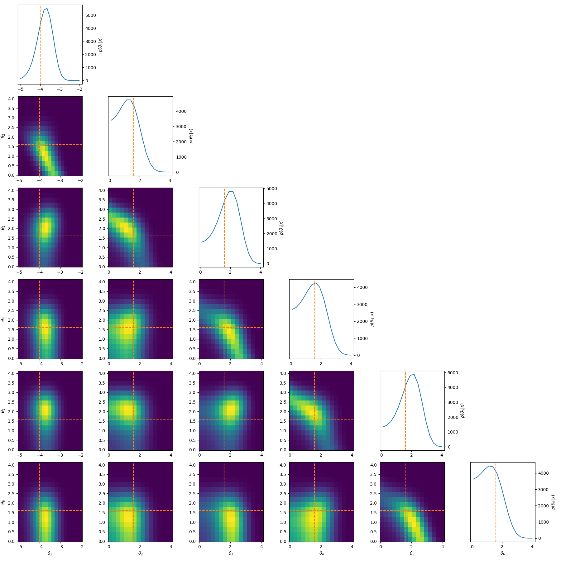
\[\begin{align} \mu_1 = \mu_{\text{min}} + \beta_1 &\cdot (\mu_{max} - \mu_{min}) \\ \mu_2 = \mu_1 + \beta_2 &\cdot (\mu_{max} - \mu_1) \\ \mu_3 = \mu_2 + \beta_3 &\cdot (\mu_{max} - \mu_2) \\ &\vdots \\ \mu_{N} = \mu_{N-1} + \beta_{N} &\cdot (\mu_{max} - \mu_{N-1}). \\ \end{align}\]Using this we get the following posteriors.
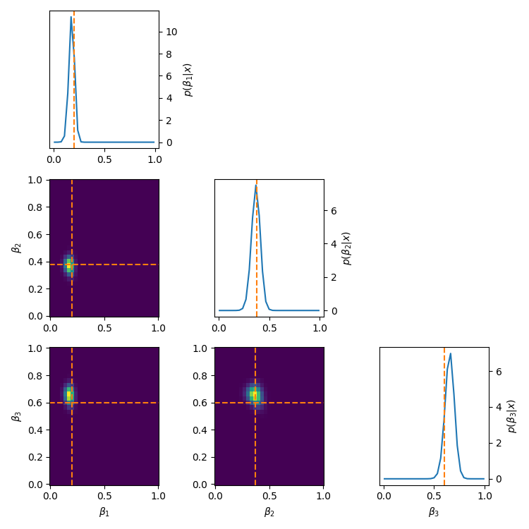
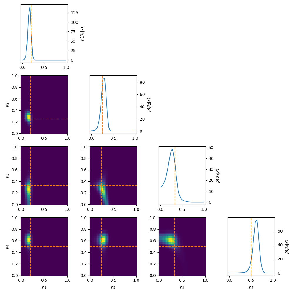
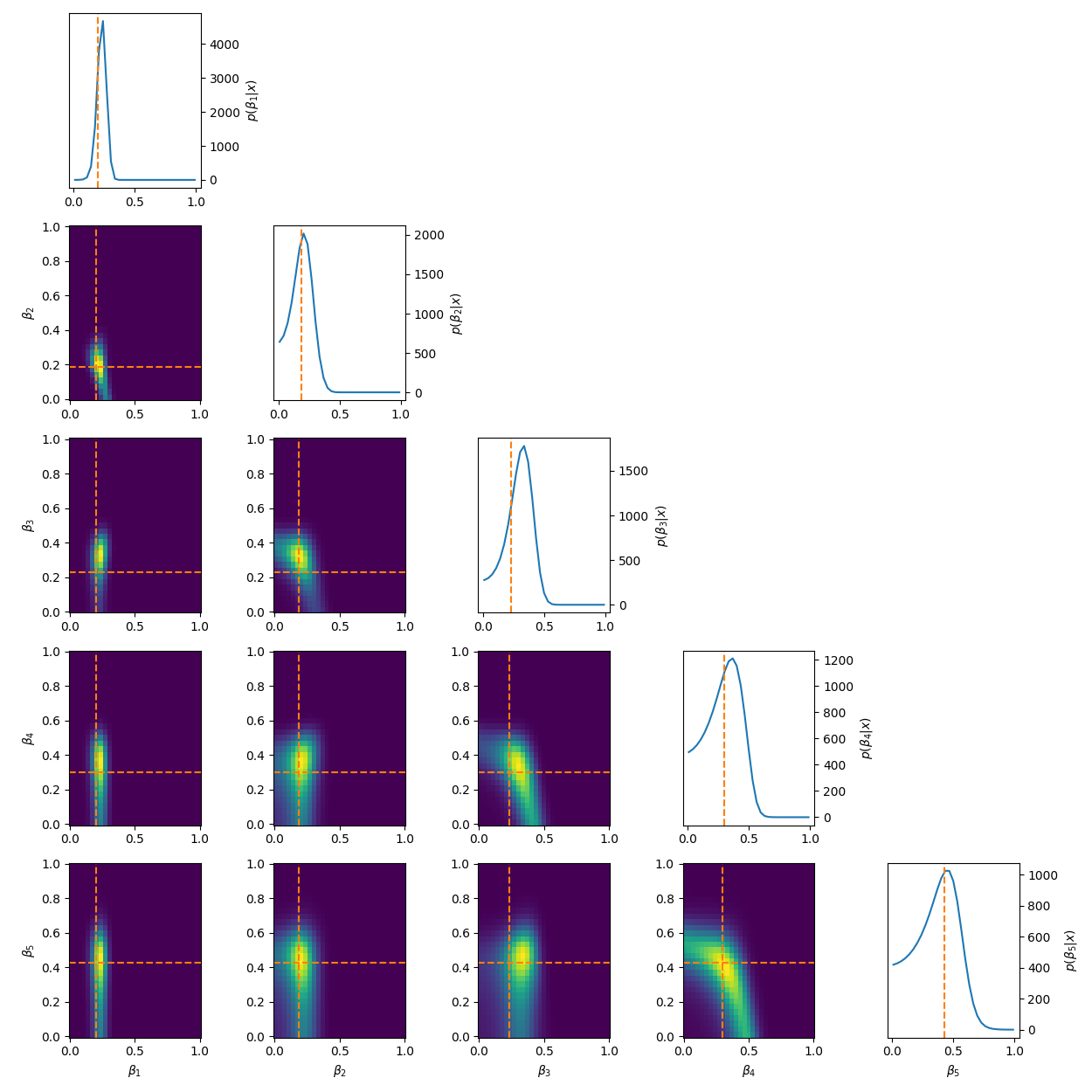
Quite often these methods make the whole setup very sensitive to the first parameter, or in general, enforces more dependency on the ‘leftmost’ parameters compared to the ‘right’. You can see this quite clearly for the five-component stick-breaking posterior. As you go down the parameter space, the width of the posterior noticeably increases. It is also worth mentioning that if one transforms back to the original coordinate system that implicitly the hard boundaries are still there, it’s just that the issues stemming from it are minimised.
In essence, there’s no such thing as a free lunch, but the above possibly reduces the cost and can turn virtually intractable problems tractable.
Possible RJMCMC Between Model kernel methods
Group A: Classical hand-designed moves
1. Birth/Death moves
The simplest set of proposal moves are birth and death moves, that as the name describes “births” a new parameter from some distribution and adds it to the current set of parameters, and the reverse of “death” move randomly picks a parameter from the current state then deletes it.
More formally, if we’re transitioning from model \(k\) with the latest sample \(\theta_k\) then with birth and death moves we either add a parameter \(u_k\) generated from some distribution \(q_k(\cdot)\) or delete a parameter either from the end of our parameter set or randomly within it. Any move pair must be constructed so that they are exact reverses of one another.
And the jacobian of the birth/death transformations \(g\) is then just the identity.
Additionally though, along with being the simplest, they are also typically the worst when it comes to acceptance probability and mixing rates. The random addition of a component leads to a very noisy representation of the posterior. So, even if there are very obviously three gaussians in your example (shown in the application section below) then this proposal type can still not recover the distribution well because the addition of the new parameter doesn’t take in anything about the distribution at all and just shoves a new component in there, probably doesn’t have enough time to converge on something nice, and then we jump away again.
This is why basically every other kind of ‘birth’ move in the follow move types use the current set of samples or posterior information to propose a new component or moves between models.
Gaussian Mixture Application
Below are some GIFs showing the RJMCMC sampling process when using a Metropolis-Hastings ‘within-model’ kernel and a birth/death ‘between model’ kernel where we make a between-model move roughly 25% of the time (a hyperparameter you can pick).
Here’s a slow version so you can analyse individual steps initialising at the true values to make my life easier and to not have to worry about burn-in. You can hopefully see that the gaussians come in and out of existence when making ‘between-model’ proposals.
And then a faster version with some stride between the frames so you can see what the whole process builds up to.

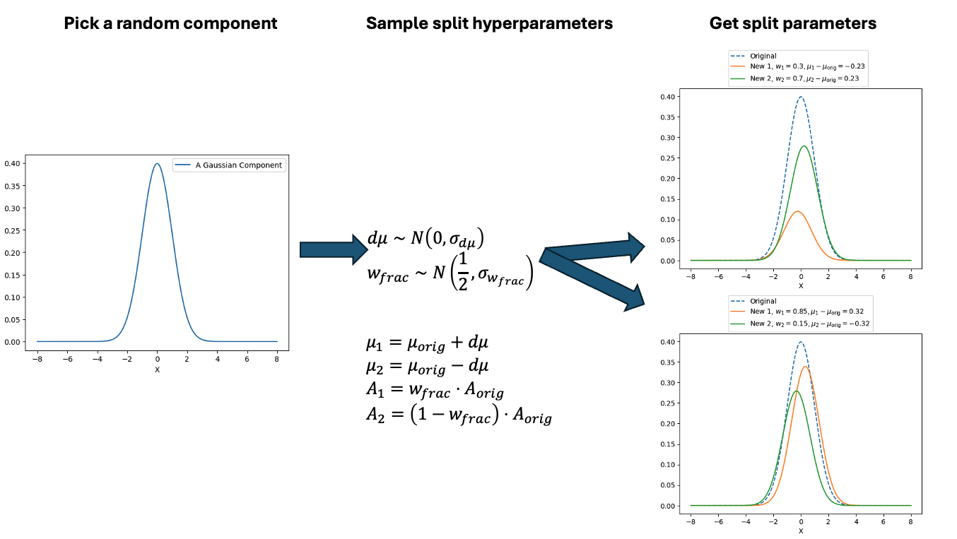
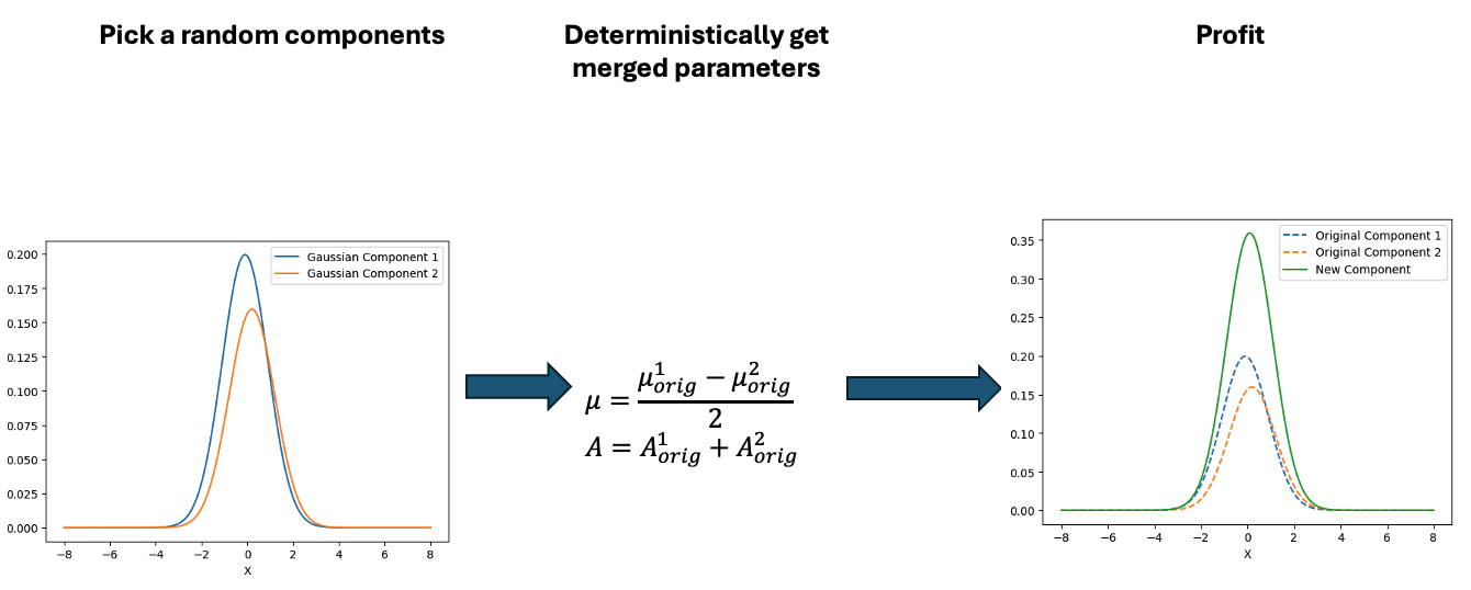
2. Split/Merge moves
Split and merge moves are just a single step more sophisticated than simple birth and death moves. The idea is that you use the auxiliary parameters to either combine or split your current set of parameters. You can think of it being designed to overcome one of the main weaknesses of simple birth/death proposals:
randomly creating entirely new structure is usually very very bad.
So we use the auxiliary parameter to try to re-structure the information that is already there.
Suppose the current model contains a component:
\[(\mu, w, \sigma)\]and we wish to split it into two components:
\[(\mu_1, w_1, \sigma_1) \;\;\; \textrm{and} \;\;\; (\mu_2, w_2, \sigma_2).\]And to be fancy we’ll demonstrate two methods for doing the split and merge moves using auxiliary parameters sampled from either a beta distribution or uniform distribution or the like.
\[(u_1, u_2, u_3)\]Then,
\[\begin{align} &w_1 = u_1, &w_2=u_2, \\ &\mu_1 = \mu - u_2, &\mu_2=\mu+u_2. \end{align}\]The auxiliary variables therefore determine:
- how the weight is divided,
- how far apart the new means are,
- and optionally how variances are perturbed.
The reverse merge move reconstructs the original component by adding the components back together (\(w_1 + w_2 = w\) and \(\mu_1 + \mu_2 = \mu\)).
Gaussian Mixture Application
Similar to above we can see this action with a gaussian mixture example where the split and merge moves are described in the two diagrams below. (The \(w_\text{frac}\) is clipped to be between 0 and 1)
With this between model kernel setup we can then apply this to our GMM example as above.
And then a faster version with some stride between the frames so you can see what the whole process builds up to.
You can hopefully see (depending on whether the GIFs load…) that as the number of components increase the distribution of points in the model become more extended in amplitude, as with more components we get more freedom with allocating probability mass. e.g. One could have 4 components not contribute a bunch or one that does quite a bit, or a roughly equal distribution of amplitudes or anything and everything inbetween.
This also leads to more issues of label switching as the distributions veer closer together. e.g In the 6 component model, many of the different component points start overlapping (this is not specific to the split/merge proposal method, you can see a similar thing happening in the birth/death). This motivates the use of some order statistics which I haven’t implemented so far, but is as described above where one fits for the differences between means instead of the means themselves (specifically I look at the log differences such that when I transform it automatically enforces positive-definiteness).
And then a faster version with some stride between the frames so you can see what the whole process builds up to.
It’s a bit hard to tell from the plots above what effect this has besides that it seems to have slightly nicer distributions for both the amplitude, means and model distribution.
3. Independence proposals (a.k.a. “centred” a.a.k.a “global” jumps)
Birth/death and split/merge proposals construct new parameters as explicit transformations of the current state. While this preserves local structure, it also means the chain typically explores model space incrementally.
Independence proposals throw this out the window and go in the opposite direction. Instead of constructing the new state as a local transformation of the current one, we instead propose an entirely new parameter vector directly from some distribution: \(\theta_{k'}' \sim q_{k'}(\theta_{k'})\).
The proposal is therefore basically independent of the current state, which is why these are called independence proposals. They are also often called global jumps because they allow the sampler to move large distances through parameter space in a single step5.
The acceptance probability becomes,
\[\begin{align} \alpha = \min\left\{1, \frac{\pi(k', \theta_{k'}') q(k' \rightarrow k)q_k(\theta_k)}{\pi(k, \theta_{k}) q(k \rightarrow k')q_{k'}(\theta_{k'})} \right\}. \end{align}\]Conceptually, this reduces RJMCMC to something much closer to ordinary Metropolis-Hastings operating over a collection of models. Independence proposals as I’ve described them sound pretty inefficient though. If we completely ignore the current state, why should the proposal land anywhere useful?
TLDR it’s because the proposal distribution itself can contain posterior information.
The key idea is that instead of carefully engineering a transformation \(g_{k\rightarrow k'}\), we instead try to directly approximate the posterior distribution of the target model.
If the proposal distribution is close to \(q_{k'}(\theta_k\vert k' ) \approx \pi(\theta_{k'}' \vert k', \mathcal{D})\), then proposed states are already likely to lie in high posterior-density regions, which can dramatically improve between-model mixing.
In essence, compared to split/merge and basic birth/death, independence proposals for for global exploration instead of locally motivated moves. This can dramatically improve mixing if the proposal distribution is good. Though of couse, if the proposal is poor, acceptance rates are as shit as you would expect.
Posterior-informed proposals
In practice, independence proposals are often constructed using:
- Gaussian approximations,
- Gaussian mixtures,
- variational inference,
- kernel density estimates,
- or normalising flows.
Typically one first performs within-model sampling, then fits an approximation to each conditional posterior \(\pi(\theta_k, k\vert\mathcal{D})\) and finally uses these approximations as proposal distributions during between-model jumps.
This can improve acceptance rates enormously, especially in high-dimensional problems where naive birth/death proposals perform poorly.
Gaussian Mixture Application
Here’s a short version of this concept once again applied to the GMM example, no order statistics are enforced, and the ellipses in the background are representative of the 1- and 2-\(\sigma\) credible intervals for the profile conditional posterior distributions for the repsective components (with estimates denoted with a \('\) and looking at the \(k^{\text{th}}\) model, then we are looking at \(p(\mu_i', A_i' \vert \vec{d}, {A_j ; A_j = A_j' \forall j\neq i}, k)\)).
And then an extended version so you can see what the sampler looks like when it’s progressed further.

This shows some obvious label switching, so we can also look at the same order statistic enforcement as was used for the split/merge.

And then an extended version so you can see what this version of the example looks like when it’s progressed further.

4. Linear/affine transformations with auxiliary noise
A large fraction of RJMCMC proposal mechanisms can be written in the general form (letting \(\theta_{k'}'\) contain \(u_{k'}'\) for ease of my sanity),
\[\begin{align} \theta_{k'}' = g_{k\rightarrow k'}(\theta_k, u_k) = A_{k\rightarrow k'} \begin{pmatrix}\theta_k \\ u_k \end{pmatrix} + B_{k\rightarrow k'}, \end{align}\]where:
- As above, \(u_k\) is a vector of auxiliary random variables,
- \(A_{k\rightarrow k'}\) handles dilations and shifts in relation to the previous set of parameters and the noise/dummy variables for a jump between \(k\rightarrow k'\)
- and \(B_{k\rightarrow k'}\) is a constant offset for a jump between \(k\rightarrow k'\)
This is a very general construction: birth/death, split/merge, and some other RJMCMC moves that I’ve seen (which is a limited list but still) are all special cases of affine transformations on an extended parameter space.
The main advantage is that the Jacobian is usually easy to compute. Since the transformation is linear (up to a constant offset), the Jacobian determinant is just
\[\begin{align} \left\vert\det\left(\frac{\partial g_{k\rightarrow k'}(\theta_k, u_k)}{\partial (\theta_k, u_k)} \right)\right\vert &= \left\vert\det A_{k\rightarrow k'}\right\vert \\ \end{align}\]Example 1.
An example of a standard birth move can be written as,
\[\begin{align} \theta_{k'}' &= \begin{pmatrix}\theta_k \\ u_k \end{pmatrix} \\ &= \begin{pmatrix}\mathbb{1}_{n_k} & 0 \\ 0 & \mathbb{1}_{n_{-k}} \end{pmatrix} \begin{pmatrix}\theta_k \\ u_{-k} \end{pmatrix} \\ &= \mathbb{1}_{n_{K}}\begin{pmatrix}\theta_k \\ u_{-k} \end{pmatrix}. \end{align}\]Denoting \(\theta_{k'}' = \begin{pmatrix} (\theta_{k'}')^{(1)} \\ (\theta_{k'}')^{(2)} \end{pmatrix}\) by blocks of size \(n_k\) and \(n_{-k}\) the reverse transformation is then,
\[\begin{align} \begin{pmatrix}\theta_k \\ u_{-k} \end{pmatrix} &= \begin{pmatrix} (\theta_{k'}')^{(1)} \\ (\theta_{k'}')^{(2)} \end{pmatrix}\\ &= \mathbb{1}_{n_{K}} \begin{pmatrix}(\theta_{k'}')^{(1)} \\ (\theta_{k'}')^{(2)} \end{pmatrix}. \end{align}\]One can see that,
\[\begin{align} \begin{pmatrix}\theta_k \\ u_{-k} \end{pmatrix} &= g_{k'\rightarrow k}\left(g_{k\rightarrow k'}\begin{pmatrix}\theta_k \\ u_{-k} \end{pmatrix} \right) \\ &= A_{k'\rightarrow k} A_{k\rightarrow k'} \begin{pmatrix}\theta_k \\ u_{-k} \end{pmatrix} \\ &= \mathbb{1}_{n_{K}} \begin{pmatrix}\theta_k \\ u_{-k} \end{pmatrix} \end{align}\]In essence, \(A_{k'\rightarrow k} = \left(A_{k\rightarrow k'}\right)^{-1}\) and \(B_{k'\rightarrow k} = -A_{k'\rightarrow k} B_{k\rightarrow k'} = -\left(A_{k\rightarrow k'}\right)^{-1} B_{k\rightarrow k'}\).
Example 2.
The relevant components of an example additive merge move can also be written as (rest is A parts = 1 for \(\theta_k\) dimensions)
\[\begin{align} \theta_{k'}' &= \begin{pmatrix}\theta_k + u_k \\ \theta_k - u_k\end{pmatrix} \\ &= \begin{pmatrix}\mathbb{1} & \mathbb{1} \\ \mathbb{1} & -\mathbb{1} \end{pmatrix} \begin{pmatrix}\theta_k \\ u_{-k} \end{pmatrix} \end{align}\]So \(A_{k\rightarrow k'} = \begin{pmatrix}\mathbb{1} & \mathbb{1} \\ \mathbb{1} & -\mathbb{1} \end{pmatrix}\) and \(B_{k\rightarrow k'} = 0\), and \(A_{k'\rightarrow k} = (A_{k\rightarrow k'})^{-1}= \frac{1}{2}\begin{pmatrix}\mathbb{1} & \mathbb{1} \\ \mathbb{1} & -\mathbb{1} \end{pmatrix}\).
General thought.
The real challenge is choosing \(A_{k\rightarrow k'}\), \(B_{k\rightarrow k'}\), and the proposal distribution for \(u_k\) so that proposed states land near regions of high posterior density. More sophisticated RJMCMC methods can basically be understood as increasingly clever ways of designing these transformations.
Group B: Proposals using local structure
5. Centering proposals (Brooks, Giudici & Roberts 2003)
One of the central difficulties in RJMCMC is that there is usually no natural geometry connecting parameter spaces across models. In fixed-dimensional MCMC, we rely heavily on local structure — gradients, covariance estimates, or random-walk scaling — to construct proposals that stay in regions of high posterior density.
Across models though, we can’t use this: moving from model \(k\) to model \(k'\) is a jump between spaces of potentially different dimension and overall behaviour (e.g. an extreme case might be something like jumping a simple 3D gaussian for basis function coefficients to a sphere or simplex of many more dimensions).
Centring proposals attempt to restore a notion of locality in this setting. They can be understood as a systematic way of answering the question:
“Given a particular mapping between models, how should we tune the proposal distribution so that the induced acceptance probability is locally as flat and as close to one as possible?”
and can broadly be viewed as the first explicit attempt to use local geometric information to design between-model moves.
Suppose we propose a move from model \(k\) with parameters \(\theta_k\) to model \(k'\) using a mapping
\[(\theta_{k'}, u) = g_{k\to k'}(\theta_k, u_k),\]where \(u_k\) is an auxiliary random variable as above.
A centring point is defined as a specific value \(u_k^\star\) such that the proposed state
\[\theta_{k'}^\star = g_{k\to k'}(\theta_k, u_k^\star)\]satisfies
\[\mathcal{L}(D \mid k, \theta_k) \approx \mathcal{L}(D \mid k', \theta_{k'}^\star).\]In fewer words: the proposed model configuration reproduces (approximately) the same likelihood contribution as the current state.
Importantly, this point is general not found by numerical optimisation. Instead, it is usually constructed from the model structure itself — for example by setting additional parameters to zero, merging duplicated components, or enforcing equality constraints that reduce model \(k'\) back to model \(k\).
e.g. For a more concrete example if we’re jumping from \(y(x\vert\vec{\theta}, k) = \theta_1^k x + \theta_0^k\) to \(y(x\vert\vec{\theta}, k') = \theta_2^{k'} x^2 + \theta_1^{k'} x + \theta_0^{k'}\) then if \(\theta_1^k = \theta_1^{k'}\), \(\theta_0^{k}=\theta_0^{k'}\) and \(\theta_2^{k'} = 0\) then the initial likelihood performance of the two will be exactly the same.
0th-order centring: calibrating acceptance to one
Given a centring point, we can evaluate the acceptance probability for the deterministic proposal
\[u_k = u_k^\star.\]The 0th-order method chooses the proposal scale parameters so that
\[\alpha\big[(k, \theta_k), (k', \theta_{k'}^\star)\big] = 1.\]i.e. the proposal distribution is tuned so that the chain always accepts a perfectly matched “equivalent” configuration in the new model.
The idea being that for proposals in a neighbourhood of \(u_k^\star\), they will also have high acceptance probability.
Higher-order methods: flattening the acceptance landscape
If the proposal distribution \(q(u)\) contains additional degrees of freedom (e.g. variance, covariance structure, or shape parameters), then the centring condition can be strengthened.
Instead of only matching the acceptance probability at a single point, one can impose that derivatives vanish at the centring point:
\[\nabla^n \alpha\big[(k, \theta_k), (k', g(\theta_k, u_k^\star))\big] = 0,\]for \(n \geq 1\) up to the number of free proposal parameters.
Relationship to Taylor expansions
The Taylor expansion appears when analysing how acceptance behaves away from the centring point.
Let
\[\mathcal{L}(u) = \log \alpha\big[(k, \theta_k), (k', g(\theta_k, u))\big].\]Expanding around \(u_k^\star\) gives
\[\mathcal{L}(u) \approx \mathcal{L}(u_k^\star) + \nabla L(u_k^\star)^T (u - u_k^\star) + \frac{1}{2}(u - u_k^\star)^T \nabla^2 L(u_k^\star)(u - u_k^\star).\]The centring conditions ensure that the leading-order structure of this expansion is controlled(/replicated ?), so that the acceptance probability remains relatively flat/good in a neighbourhood of the centring point.
Choosing a Gaussian proposal
\[u_k \sim \mathcal{N}(u_k^\star, \Sigma)\]amounts to tuning \(\Sigma\) so that proposals stay within this high-acceptance region.
Polynomial regression example
Conclusion
Footnotes
They don’t actually have to satisfy detailed balance, they have to satisfy global balance which is slightly broader. But detailed balance ensures global balance, and is typically easier to prove. ↩
If you look really closely there are some bits that have interesting implications for the original parameterisation that I won’t discuss. If you wanna learn more, a lot of people smarter than me can talk about it better. One resources that I came across that looks pretty good (and is free!) is the textbook “A First Course in Order Statistics” by Barry C. Arnold, N. Balakrishnan, and H. N. Nagaraja (link is to the pdf) ↩
You might notice that I don’t have a reference for this, it’s mostly anecdotal and I don’t have the time to construct a dedicated example for this. ↩
Although I’ll warn you there’s a lot of hidden stuff in this method so I’d recommend going to some dedicated sources on the subject ↩
I think ‘globe trotting’ would have also been a great name but I fear it was already taken… ↩