In this post I’m going to go through Gibbs and slice sampling, you’ve probably seen them used everywhere if you’re a statistician, but have you ever looked into why they work in detail? (UNDER CONSTRUCTION)

UNDER CONSTRUCTION UNDER CONSTRUCTION UNDER CONSTRUCTION UNDER CONSTRUCTION UNDER CONSTRUCTION UNDER CONSTRUCTION

Resources

Gibbs Sampling

• “The Gibbs Sampler Revisited from the Perspective of Conditional Modeling” - Kuo & Wang
• “Explaining the Gibbs Sampler” - Casella & George
  • This is good, but I think the way they describe Gibbs sampling in general sounds more like specifically collapsed Gibbs sampling
• “Gibbs Sampling” - Wikipedia
• “Gibbs Sampling, Conjugate Priors and Coupling” - Diaconis, Khare and Coste

Slice Sampling

• “Slice Sampling” - Wikipedia
• “Information Theory, Pattern Recognition, and Neural Networks - Lecture 13: Approximating Probability Distributions” - David Mackay

Table of Contents

1. Gibbs Sampling

2. Slice Sampling

3. Examples

4. Conclusion

1. Gibbs Sampling

I’m not gonna bore you with motivations for why Gibbs sampling is important, you’re either here because you’re either interested or being forced to be interested for whatever reason. Let’s just jump in.

1.1 The Core Idea

The core idea of Gibbs sampling is that you have access to conditional distributions of your data. Such that if the density you’re trying to explore is \(p(x_1, x_2)\) for example (\(x_1\) and \(x_2\) can be multi-dimensional if you want), then you have access to both \(p(x_1 \vert x_2)\) and \(p(x_2 \vert x_1)\) and with some initial condition, can sample \(p(x_1, x_2)\) by sampling the conditionals back and forth. An actual algorithm (however simple it may be) is given below.

Gibbs Sampling (2D / 2 Blocks)

1. Initialise:
   • Have a distribution you want to sample from up to some normalisation constant (duh) \(f(x_1, x_2)\), and it’s conditionals \(p(x_1 \vert x_2)\) and \(p(x_2 \vert x_1)\)
     • You only need to be able to evaluate the conditionals, you don’t need to evaluate \(f(x_1, x_2)\)
   • manually create a starting point for the algorithm \(X^0 = (x_1^0, x_2^0)\),
   • pick the number of samples you can be bothered waiting for \(N\)
2. For each iteration \(n\)/Repeat \(N\) times
   1. Sample \(x_1^{n+1} \sim p(x_1^{n} \vert x_2^{n})\)
   2. Sample \(x_2^{n+1} \sim p(x_2^{n} \vert x_1^{n+1})\)

Yep that’s it. An example of it in action is shown in the GIF below.

And if you want to get fancy with it, you can generalise to arbitrary dimensions/number of blocks by scanning or sampling through the dimensions.

Firstly we look at the one where scan through the dimensions. This is the most common version, where you visit every dimension in a fixed order (usually $1$ to $D$) during every iteration.

Gibbs Sampling (N-D, scan through dimensions)

1. Initialise:
   • Have a target distribution \(f(\mathbf{x})\) where \(\mathbf{x} = (x_1, x_2, \dots, x_D)\), and its full conditionals \(p(x_i \vert \mathbf{x}_{-i})\) for all \(i \in \{1, \dots, D\}\).
     • Note: \(\mathbf{x}_{-i}\) denotes all variables except \(x_i\).
   • Manually create a starting point \(X^0 = (x_1^0, x_2^0, \dots, x_D^0)\).
   • Pick the number of samples \(N\).

2. For each iteration \(n\) (Repeat \(N\) times):

   1. Sample \(x_1^{n+1} \sim p(x_1 \vert x_2^{n}, x_3^{n}, \dots, x_D^{n})\)

   2. Sample \(x_2^{n+1} \sim p(x_2 \vert x_1^{n+1}, x_3^{n}, \dots, x_D^{n})\)

   3. Sample \(x_3^{n+1} \sim p(x_3 \vert x_1^{n+1}, x_2^{n+1}, \dots, x_D^{n})\)

   …

   D. Sample \(x_D^{n+1} \sim p(x_D \vert x_1^{n+1}, x_2^{n+1}, \dots, x_{D-1}^{n+1})\) - Note: As soon as a variable is updated, its new value is used for all subsequent conditional samples within that same iteration.

Instead of updating every dimension, you pick one dimension at random to update during each step. This is often used in theoretical analysis and physics-based models.

Gibbs Sampling (N-D, Random Scan)

1. Initialise:
   • Have a target distribution \(f(\mathbf{x})\) and its full conditionals \(p(x_i \vert \mathbf{x}_{-i})\).
   • Manually create a starting point \(X^0 = (x_1^0, x_2^0, \dots, x_D^0)\).
   • Pick the number of steps \(N\).
2. For each step \(n\) (Repeat \(N\) times):
   1. Pick a dimension \(i\) uniformly at random from \(\{1, 2, \dots, D\}\).
   2. Update that dimension: \(x_i^{n+1} \sim p(x_i \vert x_1^{n}, \dots, x_{i-1}^{n}, x_{i+1}^{n}, \dots, x_D^{n})\)
   3. For all other dimensions \(j \neq i\), keep the value the same: \(x_j^{n+1} = x_j^{n}\)

General tips:

• Systematic Scan (the first one) is generally more efficient for computers because it ensures every variable gets updated regularly, which usually leads to faster “mixing” through the space.
• Random Scan is useful if you have a massive number of dimensions and updating all of them in one “iteration” is computationally too expensive, or if you want to avoid periodic patterns in your sampler.

1.2 Detailed balance

Gibbs sampling is evidently a Markov Chain, as each new set of points only depends on the previous, and is ergodic (because the conditional distributions should allow any coordinate in parameter space to be sampled), so to be a valid MCMC method we only have to show that the sampling satifies detailed balance (or the weaker condition of Global Balance).

In Gibbs sampling, we move along one “axis” (one variable) at a time. Thus, to understand the transition kernel let’s focus on the update for the \(i\)-th variable, \(x_i\) for a target distribution \(\pi\).

Let our current state be \(\mathbf{x} = (x_i, \mathbf{x}_{-i})\) and the proposed next state be \(\mathbf{x}' = (x_i', \mathbf{x}_{-i})\).

Note that only the \(i\)-th component changes. The transition kernel (the probability of moving from \(\mathbf{x}\) to \(\mathbf{x}'\)) for this step is: \(\begin{align} P_i(\mathbf{x} \to \mathbf{x}') = \pi(x_i' \mid \mathbf{x}_{-i}) \end{align}\)

Now, we check if \(\pi(\mathbf{x}) P_i(\mathbf{x} \to \mathbf{x}') = \pi(\mathbf{x}') P_i(\mathbf{x}' \to \mathbf{x})\):

Left-Hand Side (Forward Flow):

Using the chain rule \(\pi(A, B) = \pi(A \mid B)\pi(B)\):

Right-Hand Side (Backward Flow):

Together

If you look at the final expressions for both sides you find:

\(\pi(\mathbf{x}_{-i}) \cdot \pi(x_i \mid \mathbf{x}_{-i}) \cdot \pi(x_i' \mid \mathbf{x}_{-i})\).

Since the flow is equal in both directions, the \(i\)-th update satisfies detailed balance with respect to \(\pi\).

Systematic vs. Random Scan

There is a subtle distinction in how you apply these updates that affects whether the entire algorithm satisfies detailed balance.

Random Scan Gibbs:

If you pick a variable \(i\) at random to update in each step, the entire algorithm satisfies detailed balance. It is reversible.

Systematic Scan Gibbs:

If you always update \(x_1, x_2, \dots, x_d\) in a fixed order, the full cycle does not actually satisfy detailed balance (because you can’t just reverse the order and get the same transition probability).

However, even if the full cycle doesn’t satisfy detailed balance, it still satisfies Global Balance. Because each individual step \(P_i\) leaves \(\pi\) invariant (\(\pi P_i = \pi\)), their composition also leaves \(\pi\) invariant:

This is why systematic Gibbs sampling is still a valid MCMC algorithm, even though it is technically “non-reversible”. You could also define the transition kernel as the whole process of sampling with the combination of kernels proposed above (going from one vector of \(\vec{x}\) to one where every element has been sampled from a given conditional \(\vec{x}'\), basically how I implemented in the algorithm for the systematic scan) and that would satisfy detail balance. But that’s pretty much the same as the global balance condition in this case.

But it doesn’t have an accept-reject step?

The typical point for the accept-reject step in MCMC is to correct for the fact your proposal distribution or kernel (sans accept-reject) does not lead to the right target distribution. In this case, the kernel above does this already, and thus doesn’t need an accept-reject. i.e. The acceptance probability is 1. This is regardless of dimensionality or complexity, if you have the conditional distributions. This does not mean that the mixing (convergence) time is fantastic, as we’ll see below, highly correlated distributions can be tricky for Gibbs sampling.

1.4 When Gibbs Sampling Struggles

Separated modes

I’m just gonna let the GIF speak for itself here.

High correlation between parameters

Again, I’m just gonna let the GIF speak for itself here.

2. Slice Sampling

Slice sampling is an important technique that is commonly used as part of other algorithms (nowadays). For example NUTS uses a slice variable to define acceptable Hamiltonian states, which is conceptually related to slice sampling. To me, the introductory paper by Neal although exhaustive, was a little hard to follow imo.

2.1 The Core Idea

Slice sampling, to me, is basically a smart combination of Gibbs (the same as above) and Rejection sampling.

As a quick refresher for the second method, rejection sampling, samples a target distribution by uniformly sampling the volume under the density. This process if demonstrated below, using GIFs from my introductory post on the method.

Throwing away real-world limitations for a sec, the fundamental method behind slice sampling is where the user pretends that the density values themselves \(f(x)\) is a specific value of a variable \(y\) (like in rejection sampling), and then a two part Gibbs sampling where you sample a \(y\) value from between \(0\) and \(f(x)\), then you sample \(x\) by uniformly sampling \(x \sim U(S)\) where \(S = \{x: f(x) \geq y\}\). This implies a joint density \(p(x, y)\) that once one marginalises over \(y\) (or in practice throws out the samples of \(y\)) you attain \(p(x)\) (or samples representative of it, the normalised \(f(x)\)).

This may or may not immediately seem like rejection sampling, but the key point is that we don’t have an envelope distribution, in this theoretical setup there are no “rejected” samples!

Real world slice sampling is then an approximation to the above that is asymptotically correct. Below are some GIFs showing the exact case, as it’s pretty easy to figure out the interval \(S = \{x: f(x) \geq y\}\) in the case of the normal distribution. For the second plot I only show 100 of the coordinates at a time.

2.2 The Practical Algorithm

Now, in almost all interesting cases we do not have enough information to efficiently derive (or derive at all) \(S = \{x: f(x) \geq y\}\). So the question is how do we uniformly sample from \(S\) without explicitly know what \(S\) is?

Well Neal suggests 4 options (end of page 8 if you wanna double check):

1. Git good and just figure it out (although they suggest this may not be feasible)
2. If there is a hard bound on what values \(x_p\) can take, i.e. it can only be between 0 and 3, then we just sample that whole interval and reject points where \(y>f(x_p)\). But, similar to rejection sampling, this could be very inefficient. E.G. A beta distribution between 0 and 1, with an effective standard deviation of 0.01… and also doesn’t apply if the distribution isn’t bounded…
3. Estimate a width scale for \(S\), \(w\), randomly picking an initial interval of size \(w\), containing \(x_0\) (previous accepted proposal), and then expand it via a ‘stepping out’ procedure. Similar to 2 we can reject points where \(y>f(x_p)\) and possibly use that to expand our estimate of \(S\) as a stopping criterion.
4. Similar to 3, we can randomly pick an initial interval of size \(w\), and then expand it by a doubling procedure and have a similar stopping criterion.

Now, it would seem that the doubling procedure may be better in most cases as it can expand to larger sizes more quickly, making up for a potentially underestimated \(w\). However, it requires a rejection test, that scheme 3 doesn’t need/have, to ensure the transition is reversible. This added overhead means that more often than not the “step-out” scheme is used unless you are dealing with an extremely heavy-tailed distributions where a linear search would be slow enough to justify the added overhead of the doubling procedure.

On top of some rules for expanding the intervals, both schemes are made more efficient by a shrinkage step that uses rejected samples after the initial growth to, you guessed it, shrink the intervals to focus in on more relevant areas.

The general process for both schemes is detailed in Figures 1 and 2 in Neal’s paper that I’ve copy-pasted below (not including the captions, head over to the paper on page 9 if you want those).

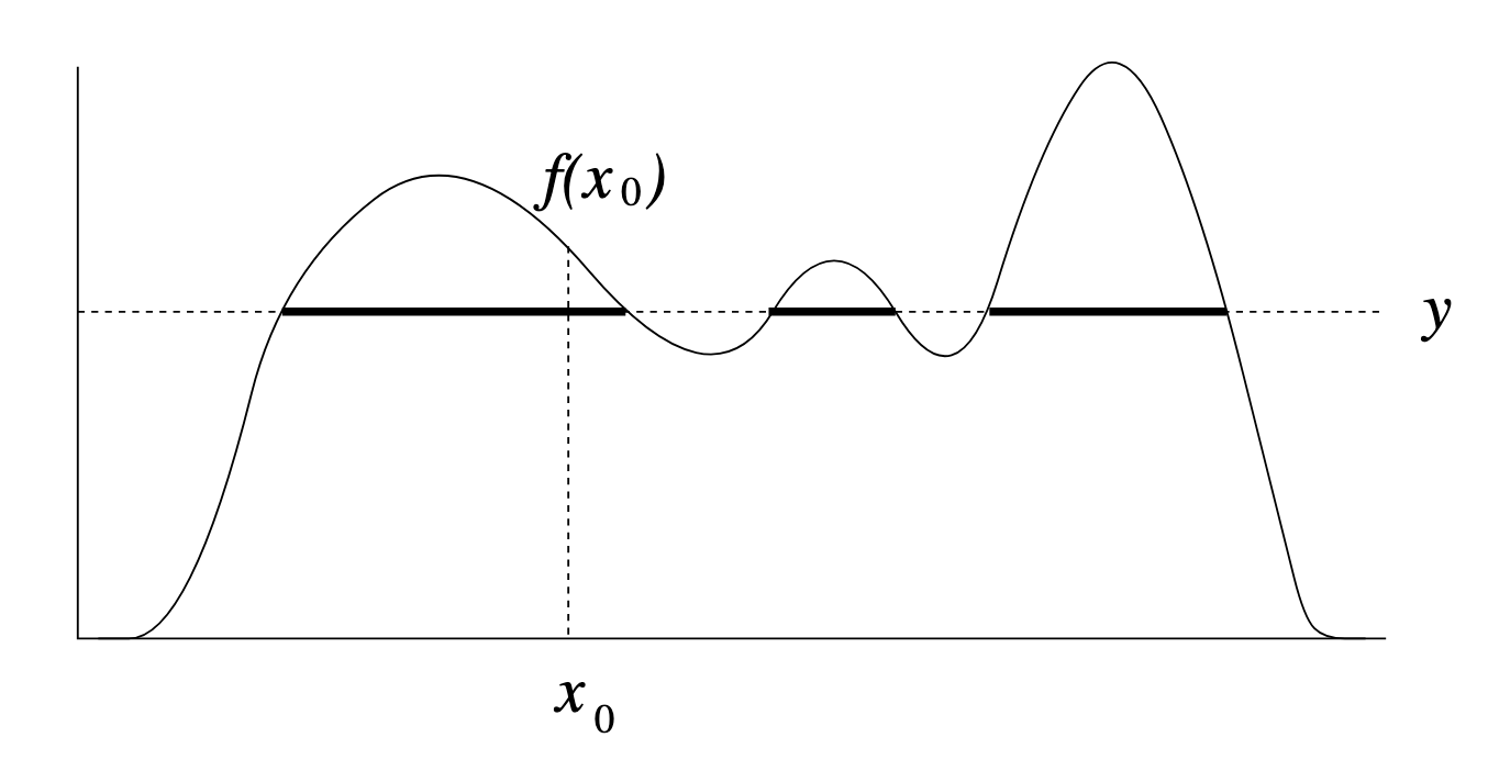
Figure 1/2 distribution

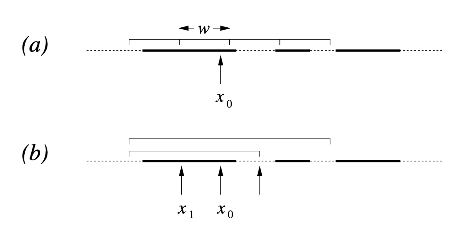
Figure 1

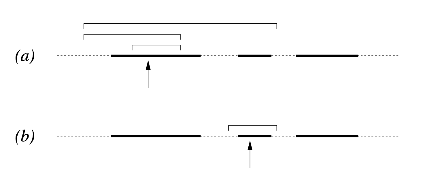
Figure 2

If this doesn’t make 100% sense at the moment that’s fine, we’ll first go through the algorithms and then a couple GIFs to see how they work in detail.

2.2.1 The “Stepping-Out” Algorithm

The stepping-out scheme is the most commonly used scheme for slice sampling because it is robust and preserves detailed balance without extra checks.

The process is as follows:

• Find the Slice: Given the current \(x_0\), pick a vertical height \(y \sim U(0, f(x_0))\). (no changes to above)
• Expand the Interval: Randomly position an interval \((L, R)\) of width \(w\) around \(x_0\).
  • If \(f(L) > y\), move \(L\) left by \(w\). If \(f(R) > y\), move \(R\) right by \(w\).
  • Repeat until both endpoints are outside the slice (i.e., \(f(L) < y\) and \(f(R) < y\)).
• Shrink and Sample: Pick \(x_{prop} \sim U(L, R)\).
  • If \(f(x_{prop}) > y\), accept it.
  • If not, shrink the interval by setting \(L\) or \(R\) to \(x_{prop}\) (whichever side \(x_{prop}\) was on relative to \(x_0\)) and try again.

Here’s the algorithm for this.

Slice Sampling: Stepping-Out Scheme

1. Initialize:
   • Have a target density \(f(x)\),
   • Propose an initial point \(x_0\),
   • Propose an estimated scale width \(w\).
   • Figure out how many iterations of the algorithm you can be bothered waiting around for \(N\).
2. For each iteration \(n\) from \(1\) to \(N\):
   • Slice: Pick a vertical height \(y \sim U(0, f(x_n))\).
   • Stepping-Out:
     • Create an initial interval \(I = (L, R)\) by picking \(U \sim U(0, 1)\) and setting \(L = x_n - w \cdot U\) and \(R = L + w\).
     • While \(y < f(L)\), subtract \(w\) from \(L\).
     • While \(y < f(R)\), add \(w\) to \(R\).
   • Shrinkage (The Proposal): Repeat until a point is accepted:
     • Sample a proposal \(x_{prop} \sim U(L, R)\).
     • If \(f(x_{prop}) > y\), Accept: \(x_{n+1} = x_{prop}\) and break.
     • Else, Shrink: If \(x_{prop} < x_n\), set \(L = x_{prop}\). Else, set \(R = x_{prop}\).

2.2.2 The “Doubling” Algorithm

The doubling scheme follows a similar logic but attempts to find the boundaries of the slice exponentially faster:

• Find the Slice: Same as above (\(y \sim U(0, f(x_0))\)).
• Double the Interval: Double the size of the interval by randomly adding the current width \(w\) to either the left or the right side.
• Acceptance Test: Because doubling can “jump” over large regions of low density and land in a separate mode, you must perform a reversibility test.
  • When a point \(x_{prop}\) is proposed, you have to verify that if you had started at \(x_{prop}\), the doubling procedure could have produced the exact same interval you are currently using.
  • Particularly, you don’t want to find that the procedure would stop before getting to the previously accepted point.
  • If this test fails, the point is rejected to prevent biasing the sampler toward wider regions of the distribution.
  • In Neal’s paper this test is shown in Figure 6.

And the algorithm…

Slice Sampling: Doubling Scheme

1. Initialize:
   • Have a target density \(f(x)\),
   • Propose an initial point \(x_0\), a
   • Propose an estimated scale width \(w\).
   • Figure out how many iterations of the algorithm you can be bothered waiting around for \(N\).
   • Figure out a limit on the number of doublings \(K\).
2. For each iteration \(n\) from \(1\) to \(N\):
   • Slice: Pick a vertical height \(y \sim U(0, f(x_n))\).
   • Doubling:
     • Create an initial interval \(I = (L, R)\) as above.
     • Repeat \(K\) times (or until both \(f(L) < y\) and \(f(R) < y\)):
       • Flip a coin.
         • If Heads, move \(L\) left by \((R-L)\).
         • If Tails, move \(R\) right by \((R-L)\).
   • Shrinkage with Reversibility Check: Repeat until a point is accepted:
     • Sample \(x_{\text{prop}} \sim U(L, R)\).
     • If \(f(x_{\text{prop}}) > y\) AND the AcceptCheck(x_prop, x_n, y, L, R, w) is true: Accept: \(x_{n+1} = x_{\text{prop}}\) and break.
     • Else, Shrink: If \(x_{\text{prop}} < x_n\), set \(L = x_{\text{prop}}\). Else, set \(R = x_{\text{prop}}\).

Func AcceptCheck(\(x_\text{prop}\), \(x_n\), \(y\), \(L\), \(R\), \(w\)):

1. Initialize:
   • Let \((\hat{L}, \hat{R}) \leftarrow (L, R)\) .
   • Set rejected = False.
2. While \(\hat{R} - \hat{L} > 1.1w\):
   • M \(\leftarrow\) \((\hat{R} + \hat{L})/2\)
   • if \(x_n < M\) and \(x_{\text{prop}} \geq M\) or \(x_n \geq M\) and \(x_{\text{prop}} \lt M\) then rejected = True
   • if \(x_\text{prop} < M\) then \(\hat{R} \leftarrow M\) else \(\hat{L} \leftarrow M\)
   • if rejected and \(y \geq f (\hat{L})\) and \(y \geq f (\hat{R})\) –> new point is not acceptable
3. Return not(rejected)

2.2.3 Final thoughts on the algorithms

Notice that in step 3 of both algorithms, if we pick a point outside the slice, we don’t just throw it away and stay at \(x_0\) (like in Metropolis-Hastings). We use that “failed” point to define a new, smaller boundary.

This means the sampler learns the shape of the slice during every single iteration. If \(w\) was way too large, the shrinkage step quickly brings it down to size.

This makes slice sampling much more stable than standard Metropolis-Hastings, where a bad proposal width \(w\) can lead to an acceptance rate of 0% and a stalled chain. And I think is one reason why slice sampling was later used as part of HMC-NUTS.

2.3 Are they valid MCMC algorithms?

Ergodicity

Under mild regularity conditions (connected support, positive density on compact subsets, etc.), univariate slice sampling is irreducible and aperiodic.

Detailed Balance

1. The Stepping-Out Procedure

In the case of the ‘stepping-out’ procedure, the probability of transitioning from \(x\) to \(x'\) entirely depends on the interval \(I\) being chosen.

Letting \(P(I\vert x, y)\) be the probability of expanding to interval \(I\) given starting point \(x\). Because the expansion happens in discrete steps of \(w\) and the initial placement is \(U(0, w)\), any interval \(I\) that could be generated from \(x\) and contains \(x'\) could also be generated if you started at \(x'\) and moved toward \(x\).

If \(x, x' \in I\) and the stepping-out condition is met for both ends of \(I\), the expansion process is identical regardless of where within \(I\) you started thus \(P(I\vert x, y) = P(I\vert x', y)\)

Since the proposal \(x'\) is uniform within the slice-restricted interval, the transition densities are equal, and detailed balance holds for the stepout procedure (and any other conditions are satisfied in accordance with it being a specific case of Gibbs sampling).

2. The Doubling Procedure

Simple doubling doesn’t automatically satisfy detailed balance, because it’s possible to reach an interval \(I\) from \(x\) that couldn’t be reached from \(x'\).

To fix this, Neal (2000) introduced an acceptance test, i.e. the AcceptCheck function above.

A transition from \(x\) to \(x'\) is only allowed if \(x'\) could have produced the same interval \(I\) using the same doubling sequence.

Let \(S\) be the subset of the interval \(I\) that is “admissible.” For detailed balance to hold:

• The slice level \(y\) is chosen uniformly.
• The probability of picking \(I\) from \(x\) must equal the probability of picking \(I\) from \(x'\).

If the doubling procedure produces an interval \(I\) from \(x\), we check if \(x'\) is “constrained.”

Simulating the doubling process starting from \(x'\), we see if it ever produces an interval that excludes the original \(x\).

If it does, the move is rejected. This “symmetry correction” ensures that \(P(x \to x' \vert y) = P(x' \to x \vert y)\).

Because the density \(\pi(x, y)\) is constant (uniform) over the slice, the equality of transition probabilities directly satisfies the detailed balance equation (and any other conditions are satisfied in accordance with it being a specific case of Gibbs sampling).

2.4 Extensions and Variants

The above slice sampling details are from the perspective of single variable sampling. There are various extensions to this method to enable multivariate density sampling. I will put the general descriptions, algorithms and representative gifs for how the sampling methods progress, but will otherwise leave to the reader to refer to Neal (2000) or the multivariate methods section of the Slice sampling Wikipedia page (although the proofs are similar/the same). Also presume not gradient information.

Multivariate slice sampling (hyperrectangle)

The basic form of Multivariate slice sampling is to construct hyperrectangles¹ in place of the intervals in the univariate case. In absence of any stepping out or doubling procedure for simplicity (although as far as I know usual implementations just do the above for each dimension), a rudimentary algorithm (adapted from Neal (2000)) is shown below.

Multivariate Slice Sampling: Hyperrectangle Scheme

1. Initialize:
   • Have a target density \(f(\vec{x})\),
   • Propose an initial point \(\vec{x_0} \in \mathbb{R}^n\),
   • Propose estimated scale widths \(\vec{w}\) (one for each dim of \(\vec{x}\)).
   • Figure out how many iterations of the algorithm you can be bothered waiting around for \(K\).
2. For each iteration \(k\) from \(1\) to \(K\):
   • Slice: Pick a vertical height \(y \sim U(0, f(\vec{x}_n))\).
   • Create an initial interval \(H = (L_1, R_1) \times (L_2, R_2) \times ... \times (L_n, R_n)\) by picking \(U_i \sim U(0, 1)\) and setting \(L_i = x_i^{k-1} - w_i \cdot U_i\) and \(R_i = L_i + w_i\).
   • Shrinkage and sampling:
     • Sample a proposal:
       • For \(i\) from \(1\) to \(n\):
         • \(U_i\) \(\sim U(0, 1)\)
         • \(x_i^\text{prop}\) \(\leftarrow L_i + U_i \cdot (R_i - L_i)\)
     • If \(f(x_i^\text{prop}) > y\), Accept: \(x_i^{k} = x_i^\text{prop}\) and break.
     • Else, Shrink: If \(x_i^{prop} < x_i^{k-1}\), set \(L_i = x_i^\text{prop}\). Else, set \(R_i = x_i^\text{prop}\).

In essence, we construct intervals in the exact same way as before for the univariate case, one dimension of \(\vec{x}\) at a time, and then shrink these intervals when a point is rejected. Examples of this process are shown below: one for showing the steps, and then the other two are sped up with different choices of \(\vec{w}\) (to show the importance of the stepping out/doubling schemes that I’m not including here).

Reflective Slice Sampling

I had a bit of trouble finding references for this one outside of Neal (2000), but reflective slice sampling is another commonly used method.

The main draw for reflective slice sampling is that while the hyperrectangle approach is straightforward, it struggles when variables are highly correlated (i.e., the “slice” is a long, thin diagonal ellipsoid, the same thing that standard Gibbs sampling struggles with above). In these cases, the axis-aligned box is no bueno, and the sampler gets stuck taking tiny steps.

Reflective Slice Sampling solves this by moving along a straight line (a ray) and “bouncing” off the boundaries of the slice. Instead of shrinking a box, we maintain our momentum.

For some intuition, imagine a particle moving inside the slice. When it hits the “wall” (where \(f(x) < y\)), we don’t stop; we calculate the gradient at that boundary and reflect the particle’s velocity vector, like a billiard ball in pool.

Multivariate Slice Sampling: (Idealized) Reflection Scheme

1. Initialize:
   • Have a target density \(f(\vec{x})\) and its gradient \(\nabla f(\vec{x})\),
   • Propose an initial point \(\vec{x}_0 \in \mathbb{R}^n\).
   • Propose a total travel distance (step size) \(w\) (not a vector, a scalar).
   • Figure out how many iterations of the total algorithm \(K\) you can be bothered to wait for.
   • Figure out how many steps in a slice trajectory \(M\) you can be bothered to wait for.
2. For each iteration \(k\) from \(1\) to \(K\):
   1. Pick a vertical height \(y \sim U(0, f(\vec{x}_{k-1}))\).
   2. Pick a random direction/momentum vector \(\vec{p}\) from rotational symmetric distribution (e.g. standard multivariate normal) and make it a unit vector.
      • Let first position of the below loop to be \(\vec{x}_{m=0} = \vec{x}_{k-1}\)
   3. (Reflection Loop) For \(m\) from \(1\) to \(M\):
      • Propose a new point: \(\vec{x}_{prop} = \vec{x}_{m-1} + w \cdot \vec{p}\).
      • If \(f(\vec{x}_{prop}) \geq y\) i.e. the move is successful. Then \(\vec{x}_{m} = \vec{x}_{prop}\).
      • Else (Hit the Boundary):
        • Set \(s=w\), \(j=1\) and \(\vec{x}_{j=0} = \vec{x}_{m-1}\) and \(\vec{x}_{j=1} = \vec{x}_{prop}\)
        • While \(f(\vec{x}_{j}) < y\):
          • Find the boundary point \(\vec{x}_b\) between \(\vec{x}_{j}\) and \(\vec{x}_{j-1}\) where \(f(\vec{x}_b) = y\).
          • Calculate the distance \(\text{dist}(\vec{x}_b, \vec{x}_{j})\) and set \(s = s - \text{dist}(\vec{x}_b, \vec{x}_{s})\).
          • Calculate the normalised inward normal \(\vec{n}\) (the unit vector in the direction of the gradient \(\nabla f\) at \(\vec{x}_b\)).
          • Reflect: Update direction \(\vec{p} = \vec{p} - 2(\vec{p} \cdot \vec{n})\vec{n}\).
          • Set \(\vec{x}_{j+1} = \vec{x}_b + s \cdot \vec{p}\)
          • Set \(j = j+1\)
        • Set \(\vec{x}_{m}=\vec{x}_{j}\)
   4. Accept: \(\vec{x}_k = \vec{x}_{M}\).

This seems pretty neat (besides the nested loop, but that will only significantly impact a run if you pick the step size to be too large hopefully), let’s code it up in the case of a standard 2D normal and make a GIF out of the process (examples shown below, hover over for different parameters).

But then there’s a particular step which in (interesting) real-world problems, is next to impossible; “Find the boundary point \(\vec{x}_b\) between \(\vec{x}_{m-1}\) and \(\vec{x}_{prop}\) where \(f(\vec{x}_b) = y\).” We could do this with the standard 2D normal because we can analytically solve for the regions given any \(y\) pretty simply.

What we can do in practice, is reflect off of the last point that was inside the boundary. Although to satisfy detailed balance, as Neal notes

“…for this method to be valid, we must check that the reverse trajectory would also reflect at this point, by verifying that a step in the direction opposite to our new heading would take us outside the slice. If this is not so, we must either reject the entire trajectory of which this reflection step forms a part, or alternatively, set \(\vec{p}\) and \(\vec{x}\) so that we retrace the path taken to this point (starting at the inside point where the reflection failed)” - Neal (2000)

i.e. If going backward in time is different to going forward, throw it out.

I then made a few GIFs of this and found the rejections looked quite boring, so instead we’ll do the other method mentioned in Neal (2000) that instead reflects based on simply the last point, i.e. the one outside the boundary. We accept a point at the end of the reflections if it lies within the boundary in the end.

“Note that for this method to be valid, one must reflect whenever the current point is outside the slice, even if this leads one away from the slice rather than toward it. This will sometimes result in the trajectory never returning to the slice, and hence being rejected, but other times, as in [Figre 14 in Neal], it does return eventually.”

Multivariate Slice Sampling: (Practical) Reflection Scheme

1. Initialize:
   • Have a target density \(f(\vec{x})\) and its gradient \(\nabla f(\vec{x})\),
   • Propose an initial point \(\vec{x}_0 \in \mathbb{R}^n\).
   • Propose a step size \(w\) (scalar).
   • Figure out how many iterations of the total algorithm \(K\) you can be bothered to wait for.
   • Figure out how many steps in a slice trajectory \(M\) you can be bothered to wait for.
2. For each iteration \(k\) from \(1\) to \(K\):
   1. Pick a vertical height \(y \sim U(0, f(\vec{x}_{k-1}))\).
   2. Pick a random direction vector \(\vec{p}\) from a rotationally symmetric distribution (e.g. standard multivariate normal) and normalise: \(\vec{p} \leftarrow \vec{p} / \|\vec{p}\|\).
      • Let first position of the below loop be \(\vec{x}_{m=0} = \vec{x}_{k-1}\).
   3. (Trajectory Loop) For \(m\) from \(1\) to \(M\):
      • Propose: \(\vec{x}_{m} = \vec{x}_{m-1} + w \cdot \vec{p}\).
      • If \(f(\vec{x}_{m}) \geq y\): the move is inside the slice. Continue.
      • Else (outside the slice):
        • Compute the normalised gradient at the outside point: \(\hat{n} = \nabla f(\vec{x}_{m}) / \|\nabla f(\vec{x}_{m})\|\).
        • Reflect direction: \(\vec{p} \leftarrow \vec{p} - 2(\vec{p} \cdot \hat{n})\hat{n}\).
        • (The particle has moved to \(\vec{x}_{m}\) regardless — it does not stay at \(\vec{x}_{m-1}\).)
   4. If \(f(\vec{x}_{M}) \geq y\): Accept \(\vec{x}_k = \vec{x}_{M}\).
   5. Else: Reject the trajectory, set \(\vec{x}_k = \vec{x}_{k-1}\) (keep previous sample).

And now some GIFs of this more practical algorithm.

4. Conclusion

Hope this post comes in handy, especially for the slice sampling which I couldn’t find a lot of resources for… As always, if something didn’t make sense, or you think the figures/GIFs could communicate a point better with some tweaks/a different figure, please shoot me an email.

For now, if you want more fun sampling stuff, I made this post as a bit of an explainer for a couple minor points in another post titled “Speeding up MCMC with Langevin and Hamiltonian dynamics and stochastic gradient estimates” which should be linked as the next post below.

Footnotes