Speeding up MCMC with Langevin and Hamiltonian dynamics and stochastic gradient estimates

96 minute read

Published: January 18, 2026

In this post I’m going to try and introduce Hamiltonian and Langevin Monte Carlo, and there stochastic gradient counterparts (among a couple other things). This post will involve a little stochastic differential calculus and some results from A Complete Recipe for Stochastic Gradient MCMC - Ma et al. (2015).

Resources

Main Resources

A Complete Recipe for Stochastic Gradient MCMC - Ma et al. (2015)
Microcanonical Hamiltonian Monte Carlo
Fluctuation without dissipation: Microcanonical Langevin Monte Carlo
“Bayesian Theory and Computation Lecture 10: Advanced MCMC” - Cheng Zhang
- Found this after making the original draft of the post but it basically follows the exact same story points… (sans a bit about SDEs)

LMC/Langevin Methods

The Motivation: Why “Random” Isn’t Enough

MCMC is one of the most revolutionary and widely used tools in a statisticians arsenal when it comes to exploring probability distributions. But despite this, it is deceptively simple and possibly doesn’t use all available information to speed up sampling. In this post we’re going to see some ways that we can possibly use some of this available information to do exactly that.

First, I’ll do a quick refresher for what Metropolis-Hasting MCMC is. If you are completely, unfamiliar with Metropolis-Hasting MCMC I’d recommend (in my completely unbiased opinion) my practical guide on MCMC and especially the resources/references within but I’ll cover the main points below.

Metropolis-Hasting MCMC (MHMCMC) comprises of three things: a (typically unnormalised) target distribution, a proposal distribution and how many iterations of the below algorithm you can bare to wait for.

Metropolis-Hastings Algorithm

Initialise:

Have a distribution you want to sample from (duh) $f(x)$,

manually create a starting point for the algorithm $x_0$,

pick a distribution $g(x\mid y)$ to sample from

pick the number of samples you can be bothered waiting for $N$

For each iteration $n$/Repeat $N$ times

Sample a new proposal point $x^*$ from the symmetric distribution centred at the previous sample

Calculate the acceptance probability $\alpha$ given as $\alpha = \frac{f(x^*)g(x_n\mid x^*)}{f(x_n)g(x^*\mid x_n)}$ (Here’s the change!)
And if the acceptance probability is more than 1, cap it at 1.

Generate a number, $u$, from a uniform distribution between 0 and 1

Accept or reject

Accept if: $u\leq\alpha$, s.t. $x_{n+1} = x^*$

Reject if: $u>\alpha$, s.t. $x_{n+1} = x_n$

This amounts to exploring a given distribution in the method indicated in the GIF below.

GIF showing the process of an MHMCMC Algorithm (with symmetric proposal making it equivalent to Metropolis MCMC)

The target distribution is the distribution that we are trying to generate samples for and all we need is a way to evaluate it up to a normalisation constant. The proposal distribution is then some other distribution, that uses the previous accepted value that we have sampled, to propose a new point (and either accept-reject based on the density ratio with respect to the previous accepted sample). This amounts to something we call a Markov Process, which can be viewed as a discrete-time stochastic or random process (we will revisit what this means later), where every sample/event only depends on the previous.

This is why Metropolis MCMC is sometimes referred to as a type of “Gaussian random walk” (in the case of a gaussian proposal distribution) or Random Walk Metropolis (RWM, as I will more generally refer to for the above types of MCMC algorithms).

These algorithms have been stupidly successful, being used from investigating the properties of stars in other galaxies to how the share prices of toy companies will vary in a given month. The key benefit to this is the ability to partially side-step the curse of dimensionality, that arises if one were to naively grid every dimension of a given distribution one wanted to investigated.

RWM works great for moderately dimensional spaces (very roughly from my experience up to 15 dimensions for non-pathological distributions) but is not able to get around the curse entirely¹.

There are two key issues that RWM struggles with in higher dimensional spaces: the way volume behaves in these spaces, and the general in-efficiency of the process as a function of dimension.

Pathological Volumes and Shells

In high dimensional spaces, very basic things one would presume about volume and space break down. e.g. A particularly fun thing that can happen regarding spheres escaping the boxes that you would think contain them is explained in this numberphile video.

The particular issue in the case of RWM algorithms is that the typical set or the space where the probability mass (for our purposes here, this is synonymous with infinitesimal integrated chunks of probability density), becomes exponentially concentrated about a sphere about the origin.

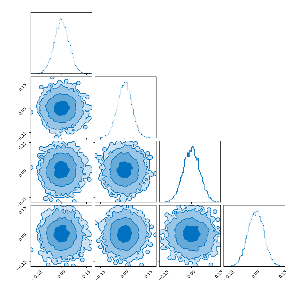
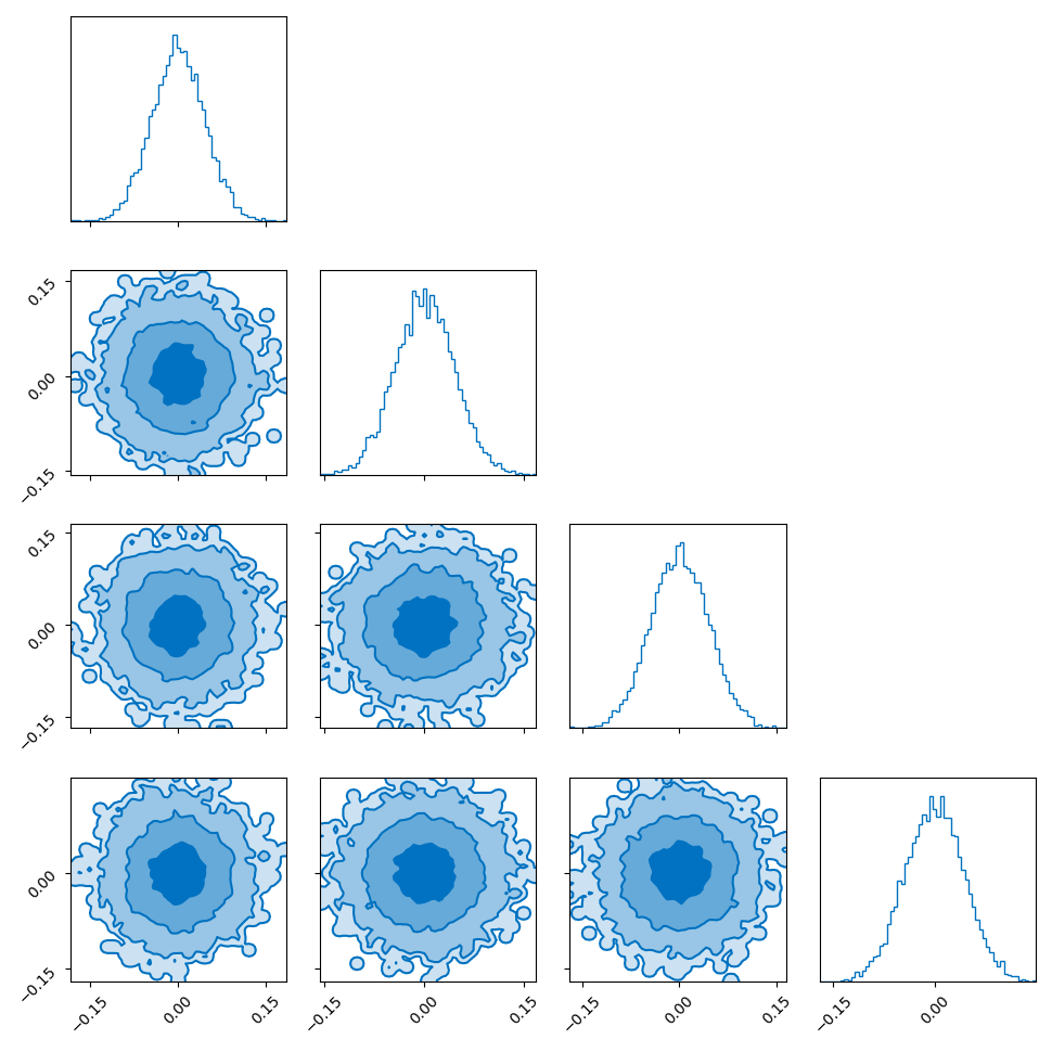
I showed the converse of this in my post on hyperspherical and hyperbolic VAEs, where if you sample uniformly on the unit sphere in high dimensions (~500), the distribution you get out in the marginals (the corner plot) is indistinguishable from those of a similarly dimensional gaussian.

Comparison of a sample distribution on a uniform sphere and normal distribution in 500-dimensional space (not necessarily in that order)

So you get this kind of Faustian bargain where you can either:

Making the step size/width of the proposal small, so that samples that are close/on the sphere stay close/on the sphere. But then exploring the hall space/distribution will be very slow, making the process take exponentially longer.
Making the step size/width of the proposal large, so you can quickly explore the whole space, but have a low efficiency of having samples fall in the typical set, making the process take exponentially longer….

Walking home drunk is not an efficient way to get home (kinda)

Closely linked to the above issue is how the efficiency of the stochastic process (sometimes referred to as a drunken walk process) scales with dimension. For a $d$-dimensional distribution the efficiency of the process assuming an target efficiency of ~0.234 (23.4\%) (refs Optimal scaling of discrete approximations to Langevin diffusions - Roberts, Rosenthal (1998), Investigating the Efficiency of the Metropolis Algorithm - Dou, Li, Wang (2024)) the optimal step size for RWM scales as $d^{-1/2}$ and efficiency (or number of steps) as $\mathcal{O}(d)$.

Viewing this process as a diffusion process, where the efficiencies relate to how long it takes to reach an equilibrium distribution or a good enough approximation of one, then leaves the door open for us to wonder if other dynamics/processes could scale significantly better?

One possible algorithm that achieves this are the so-called “Langevin algorithms” that model the process via Langevin dynamics. Roberts & Tweedie (1996) showed that the proposal distributions for Langevin-based algorithms could scale as $d^{-1/3}$ and the number of steps as $\mathcal{O}(d^{1/3})$! Which for high-dimensional sampling is a complete game changer when it comes to efficiency.

Sneak Peek: An intuitive picture of Langevin Monte Carlo

Imagine the sampling trajectories of MCMC as people trying to find their way home after a long night out. They are in their neighborhood, but they are delirious and have no sense of direction.

The RWM drunkards have lost their glasses in the mayhem of the night, and thus have completely failing eyesight. They pick a house at random nearby, stumble to the door, and are then close enough to check the house number on the door (the probability density). If that number is closer to their own address, they feel a sense of “positive feedback” and are likely to stay there for a moment. But then, forgetting everything, they stumble toward another random house. As this process repeats they have an unconcious positive feedback ‘pull’ towards the right house number. They are essentially “diffusing” through the neighborhood. Because they don’t know which way the numbers are increasing or decreasing, they spend a massive amount of time walking in circles or heading toward the wrong end of the street.

The Langevin (LMC) Drunkard is just as tired, but they’ve managed to keep their glasses on. They can actually read the street signs. They notice the house numbers are increasing as they walk East, so they purposefully start walking East (the Drift). They are still drunk, so they still trip over the curb or weave side-to-side randomly (the Diffusion), but their average movement is a direct line toward their front door.

In a 1D street, the RWM drunkard might eventually find home. But imagine a 100-dimensional neighborhood (for this I like to imagine Los Angeles in Blade Runner 2049 but when you take a step in the wrong ‘direction’ you land in Ready Player One).

The RWM drunkard is almost certain to take a step that leads them away from their house because there are so many “wrong” directions to choose from.
The LMC drunkard, even with a slight stagger, has a compass (the Gradient). They ignore the 99 wrong directions and focus their energy on the one direction that actually matters.

More formally, LMC introduces a drift into the proposal distribution or gradient flow using the gradient of the target probability density but otherwise uses the same accept-reject step as in typical MHMCMC algorithm. And even more formally … is the rest of this post.

Below is a GIF showing how RWM and LMC converge on a target (same step size, set so that RWM is purposefully bad, but even then the LMC is fine).

We will try to motivate how we construct the below algorithm and possibly generalise it?

Metropolis-Adjusted Langevin Algorithm

Initialise:

Have a target density you want to sample from $f(x)$ (known up to a normalising constant),

Define the potential energy as the negative log-density: $U(x) = - \log f(x)$,

Manually choose a starting point $x_0$,

Pick a step size $\epsilon > 0$,

Pick the number of samples to generate $N$.

For each iteration $n$ / Repeat $N$ times:

Langevin proposal steps:

Compute the gradient of the log-density at the current state: $\nabla \log f(x_n)$

Generate a proposal point $x^*$ using a drift term plus noise: $x^* = x_n + \frac{\epsilon}{2} \nabla \log f(x_n) + \sqrt{\epsilon} \eta$ where $\eta \sim \mathcal{N}(0, I)$

Metropolis Hastings correction steps:

Compute the proposal densities: $q(x^* \mid x_n) = \mathcal{N}\left(x^* ; x_n + \frac{\epsilon}{2} \nabla \log f(x_n),\epsilon I\right)$ $q(x_n \mid x^*) = \mathcal{N}\left(x_n ; x^* + \frac{\epsilon}{2} \nabla \log f(x^*),\epsilon I\right)$

Compute the acceptance probability: $\alpha = \min\left(1, \frac{f(x^*) q(x_n \mid x^*)}{f(x_n) q(x^* \mid x_n)}\right)$

Draw a random number $u \sim \text{Uniform}(0, 1)$

Accept or reject:

If $u \le \alpha$, set $x_{n+1} = x^*$

If $u > \alpha$, set $x_{n+1} = x_n$

Another Sneak Peek: An intuitive picture of Hamiltonian Monte Carlo

A much more commonly used algorithm (compared to LMC) is Hamiltonian Monte Carlo or HMC. Similar to LMC where we start thinking of the sampling procedure as some stochastic process, HMC looks at the problem as a dynamic deterministic process. They key idea being that you literally treat the problem as some ficticious physical system where the samples of the parameters in the posterior $\vec{\theta}$ are akin to position vectors, and we add some auxillary momentum vectors $\vec{r}$.

We then define a Hamiltonian that defines the system, traversing equal energy contours, such that new proposed points will have similar or higher acceptance probabilities as the initial points, with a metropolis-hasting’s-like adjustment so that the algorithm doesn’t just turn into an optimisation routine. The Hamiltonian is generally (like 99+\% of the time) as,

\[\begin{align} \mathcal{H}(\vec{\theta}, \vec{r}) = U(\vec{\theta}) + K(\vec{r}), \end{align}\]

where $U$ is our equivalent of potential energy, defined by $U(\vec{\theta}) = - \log p(\vec{\theta}, \vec{x})$, $\vec{x}$ being our data but is effectively treated as a constant here. The kinetic energy $K$ is then similarly defined as the negative of the log of the probability of a given momentum, typically chosen to just be a multivariate normal distribution with $0$ mean and unit variance. So,

\[\begin{align} K(\vec{r}) &= - \log p(\vec{r}) \\ &= - \log \mathcal{N}(\vec{0}, I) \\ &\propto - \log \exp\left(-\frac{1}{2} (\vec{r} - \vec{0})^T I^{-1} (\vec{r} - \vec{0}) \right) \\ &= \vec{r}^T \vec{r}/2. \end{align}\]

This nicely matches up with actual (classical) physical systems where the kinetic energy is $p^2/2m$.

As in classical physics we can then evolve the system according to²,

\[\begin{align} \frac{d}{dt}\vec{\theta} = \frac{\partial H(\vec{\theta}, \vec{r})}{\partial \vec{r}} \\ \frac{d}{dt}\vec{r} = - \frac{\partial H(\vec{\theta}, \vec{r})}{\partial \vec{\theta}}. \end{align}\]

If unfamiliar, part of the reason it is we model physical systems this way is because this then enforces that energy is conserved/the derivative of the total energy with respect to time is 0,

\[\begin{align} \frac{d}{dt} H(\vec{\theta}, \vec{r}) &= \frac{\partial H(\vec{\theta}, \vec{r})}{\partial \vec{\theta}} \frac{d}{dt}\vec{\theta} + \frac{\partial H(\vec{\theta}, \vec{r})}{\partial \vec{r}}\frac{d}{dt}\vec{r}\\ &= \frac{\partial H(\vec{\theta}, \vec{r})}{\partial \vec{\theta}} \frac{\partial H(\vec{\theta}, \vec{r})}{\partial \vec{r}} - \frac{\partial H(\vec{\theta}, \vec{r})}{\partial \vec{r}}\frac{\partial H(\vec{\theta}, \vec{r})}{\partial \vec{\theta}} \\ &= 0. \end{align}\]

This leads us to essentially modelling a physical system, where previously we were modelling a markov process on a probability density. The potential of the system is the negative log probability of the distribution we want, and the proposal samples are generated by traversing along equal energy contours/the paths particles would take in a physical system. There’s just a few things regard how long the paths are between proposals, how big the steps are in these traversals, monte carlo adjustments related to making a discrete approximation to a continuous system and reversing the momentum after accepting a sample.

A naive implementation is shown in the GIF below.

(Although now I realise the labels for the contours of the KDE estimate are the wrong way around…)

Some mathematical background

In this section we’ll go through the required math particularly to understand Langevin Dynamics and the Fokker-Planck Equation. If you either: are not fussed about the nitty-gritty details or are already familiar with the topics above you can skip this section. I endeavoured to make the other sections not rely on this section but I will refer back to them every now and then for details.

Stochastic Differential Equations (SDEs)

You can essentially describe SDEs as an extension to ODEs that includes some noise or stochastic component (for the purpose of this blog post at least).

In essence, where you would have an ODE described by:

\[\begin{align} \begin{cases} \frac{d\vec{x}}{dt}(t) = b(\vec{x}(t)) & (t\geq 0) \\ \vec{x}(0) = \vec{x}_0 \end{cases} \end{align}\]

that described some smooth trajectory $\vec{x}(t)$ ($\vec{x}$ some stand-in for some arbitrary quantity) or progression of states for times $\geq 0$, that may look like the following for example,

If you add a noise component, that may look like,

such that the system can only now be adequately described by,

\[\begin{align} \begin{cases} \frac{d\vec{y}}{dt}(t) = b(\vec{y}(t)) + B(\vec{y}(t)) \vec{\xi}(t) & (t\geq 0) \\ \vec{y}(0) = \vec{y}_0 \end{cases} \end{align}\]

where $B:\mathbb{R}^n \rightarrow \mathbb{M}^{n \times m}$ (space of $n\times m$ matrices) and $\vec{\xi}(t)$ an $m$-dimensional vector function that would be described as ‘white noise’ (with now $\vec{y}$ now some stand-in for some arbitrary quantity to highlight the difference with $\vec{x}$ the smooth ODE result).

The white noise term is often replaced with the time derivative of a “Wiener process”/brownian motion process³ $\frac{dW}{dt} = \vec{\xi}(t)$ which then allows us to express the above in differential form as below.

\[\begin{align} \begin{cases} d\vec{y} = b(\vec{y}(t)) dt + B(\vec{y}(t)) dW(t) & (t\geq 0) \\ \vec{y}(0) = \vec{y}_0 \end{cases} \end{align}\]

Thus the general solution of the SDE is then “just”,

\[\begin{align} \vec{y}(t) = \vec{y}_0 + \int_{s=0}^{s=t} b(\vec{y}(s)) ds + \int_{s=0}^{s=t} B(\vec{y}(s)) dW(s). \end{align}\]

But for anyone vaguely familiar with Brownian motion it is everywhere continuous and nowhere differentiable so $\frac{dW}{dt}$ for sure doesn’t really exist. So:

What even is $dW$?
What does $\int_{s=0}^{s=t} dW(s)$ mean?

What even is $dW$?

Skipping some motivation and background we can define the process $W(t)$ as:

Wiener Process Definition.

The process $W$ has the initial condition $W(0) = 0$,

$W(t) - W(s) ~ \mathcal{N}(0, t-s), \forall \; t\geq s \geq 0$,

$\forall t$ where $0 \lt t_1 \lt t_2 \dots \lt t_n$, the increments/differences $W(t_{j+1}) - W(t_j)$ are independent

Here $W(t)$ is basically just describing any process where some particle/object/thing jiggles, such that it’s particular position at any point in time can be represented probabilistically as some gaussian with variance given as the difference in time between either the starting time or some reference point.

In standard calculus, $dx$ is just the infinitesimal change in $x$. In our stochastic world, $dW$ is more of an infinitesimal shock. It’s not exactly a slope; it’s a tiny, random kick or variance in the process.

But similar to the “smooth” calculus $dx$, we take the limit $\Delta t \to dt$ with $\Delta W = W(t + dt) - W(t)$, to get some of the properties of the “stochastic differential” $dW$:

Expectation is zero: $E[dW] = 0$. On average, the noise doesn’t “push” the particle in any particular direction, on average it stays where it started.
The “Square” Rule: In standard calculus, $(dt)^2$ is so small we often ignore it. But for a Wiener process: $(dW)^2 \approx dt$ (more strictly $E[(dW)^2] = dt$ but ).

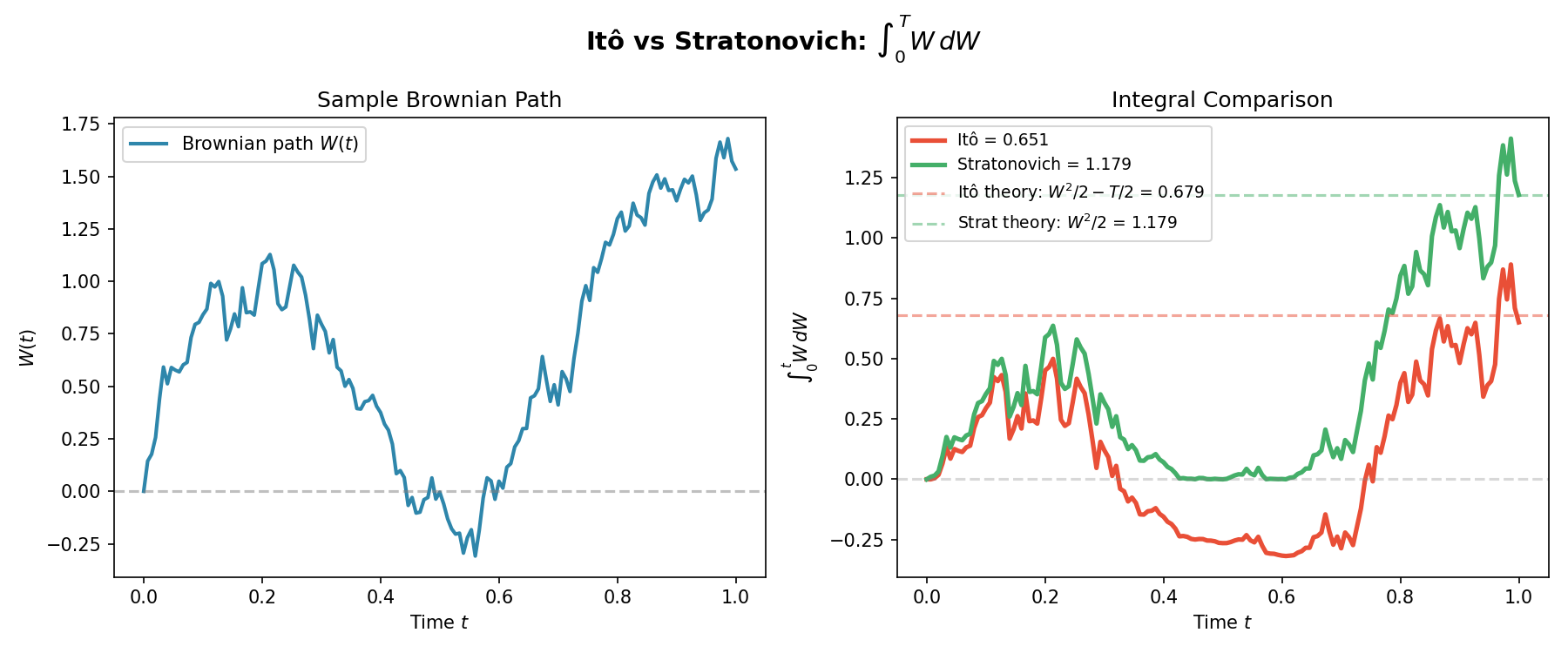
Stochastic Integrals: Itô Calculus vs. Stratonovich / What does $\int_{s=0}^{s=t} dW(s)$ mean?

If we try to solve the integral term $\int B(y(s)) dW(s)$ using standard Riemann sums, things don’t work out very well because the path of $W(t)$ is so jagged—it has infinite variation—the answer depends on where in the rectangle you measure the height.

We have two main choices, which essentially boil down to: “When does the noise hit?”

1.The Ito Integral (Common Financial/CS Choice)

In the Itô (or the incorrectly spelled Ito as you will likely note after this section, is named after the mathematician Kiyosi Itô) interpretation, we evaluate the function at the beginning of the time step, kind of like if you were trying a model a situation in the wild, you only have the information up to the current timestep, you don’t know the information in half a timestep’s time, let alone a full one.

\[\int_0^t B(s) dW(s) \approx \sum_{i} B(t_i) (W(t_{i+1}) - W(t_i))\]

This is the standard for finance and computer science. It has the “martingale” property: the noise at the current step is independent of the state, meaning you can’t use the noise to “peek” into the future (Sean Dineen’s textbook on probability and SDEs has a more nice in-depth explanation for this). However, it doesn’t imply the typical chain rule of standard calculus.

To differentiate functions of stochastic processes, you need Ito’s Lemma (kind of like the Taylor Series for SDEs):

\[df = \left( f'(y)b(y) + \frac{1}{2}f''(y)B(y)^2 \right)dt + f'(y)B(y)dW\]

Remembering that $(dW)^2 \approx dt$, we get extra terms that wouldn’t exist in normal calculus.

2.The Stratonovich Integral (The “Physics” Choice)

For the Stratonovich Integral⁴, we evaluate the function at the midpoint of the time step:

\[\frac{t_i + t_{i+1}}{2}.\]

Giving the definition of the integral to be:

\[\int_0^t B(s) dW(s) \approx \sum_{i} B\left( \frac{t_i+ t_{i+1}}{2}\right) (W(t_{i+1}) - W(t_i)).\]

This formulation preserves standard calculus rules (the chain rule works as expected!), making it popular in physics.

However, it secretly looks into the future (the midpoint uses information from $t_{i+1}$), making it computationally awkward for simulations where causality matters.

Again, kind of by construction, for a discrete process like making investments in a finance, you are stuck in the present, you shouldn’t be using information of the future.

TL;DR: We will stick to Ito for simplicity in sampling algorithms, but we have to be careful with our calculus rules. Below is a gif showing some an example difference between the two for the same path.

And then just for the last frame so you don’t have to watch the gif over and over again.

The Langevin SDE: Combining Deterministic Drift and Random Fluctuations

Now we can define the specific SDE that is behind the Langevin dynamics introduced above!

Langevin Dynamics models the movement of a particle in a fluid. It is subject to two forces:

Drag/Friction: It wants to stop moving or settle into a low-energy state.
Thermal Fluctuation: The random collisions with fluid molecules (the “noise”) kicking it around.

In the context of sampling (e.g., finding the parameters of a Bayesian model), we treat the “energy landscape” as the negative log-probability of our target distribution (as I defined above for the sneak peak in HMC).

We want the particle to settle in the high-probability regions (low energy) but keep jiggling to explore. We use the Overdamped Langevin Equation, where we assume the friction is so high we can ignore mass and momentum⁵.

The velocity is proportional to

\[dY_t = -\nabla U(Y_t) dt + \sqrt{2D} dW_t,\]

which is dependent on:

the state/position $Y_t$
the Drift: $-\nabla U(Y_t)$. This pushes the particle downhill toward the minimum of the potential energy $U(x)$.
and finally the diffusion $\sqrt{2D} dW_t$: This is the thermal noise that prevents the particle from just getting stuck in the nearest local minimum. i.e. $D$ controls the “temperature” and is assumed to be a constant diagonal matrix (with the square root an element-wise operation or D is just a constant $\in \mathbb{R}$)

A gif showing the combination of the effects is below.

The Fokker-Planck Equation: “Flowing” Probability?

So far, we’ve looked at the path of a single particle. But since the movement is random, what if we ran this simulation a million times? Or what if we had a million particles? Or more simply, how do we know if a distribution is the steady-state or final solution of our dynamics?

But since the movement is random, looking at one squiggly line doesn’t tell us what we need to know.

Instead of tracking the position of one particle, let’s track the probability density $p(x, t)$. This tells us the probability of finding the particle at position $x$ at time $t$.

If we want to see how this probability cloud evolves over time, we need a Partial Differential Equation (PDE).

For this we can imagine that the probability is like a fluid: it cannot be created or destroyed, it can only flow from one place to another.

This is mathematically described by the Continuity Equation:

\[\frac{\partial p(x, t)}{\partial t} = -\nabla \cdot J(x, t)\]

Where $\frac{\partial p}{\partial t}$ is the change in probability at a specific spot, $J$ is the Probability ‘Flux’ (or ‘current’) describing where the probability is flowing, $\nabla \cdot J$ is the the ‘divergence’, measuring how much “stuff” is leaving a point (but can also be negative, so also measures stuff entering a point).

More simply the equation says: “The amount of probability at a point changes only if probability flows in or out of that point.” Nothing will magically appear or dissapear and the sum of derivatives of the flux of stuff with respect to space is directly proportional to the time derivative of the total amount of stuff moving in and out the neighbourhood of a given point.

I tried to “GIF”-ify this, but I’m not sure how effective it is. There are two plots below showing a ball of ‘probability’ moving through a box/space (you can think of this as the neighbourhood of a given point) and then an abstract fluid.

ball of stuff

abstract fluid

Although while trying to find some inspiration for GIFs to make that would be better than the above or require me to learn manim, I found this meme where the bit this guy is writing is closely related to what we’re doing here. Which I think is as good as I can do 😂 (for those wondering, no it is not simple math…).

For a better resource on the integral formulation and differentual formulation of the continuity equation (we are using the differential form) I’d recommend this video by Steve Brunton.

In our Stochastic Differential Equation, the flux $J$ is made of two competing parts:

The ‘Advective’ Flux (Drift): The deterministic force $b(x)$ pushing the particle.$J_{\text{drift}} = b(x) p(x, t)$. This is the “River” part. If you just had this (no noise), you would recover the general form of Liouville’s Equation for deterministic flow (basically just the continuity equation above for deterministic processes).
The ‘Diffusive’ Flux: The random noise spreading things out. By Fick’s Law, stuff naturally flows from high concentration to low concentration. $J_{\text{diffusion}} = - \frac{D(x, t)}{2} \nabla p(x, t)$. This is the “Dye Spreading” part.

If we just plug our total flux $J = J_{\text{drift}} + J_{\text{diffusion}}$ back into the continuity equation, we get the Fokker-Planck Equation:

\[\frac{\partial p}{\partial t} = -\nabla \cdot \left[ \underbrace{b(x) p}_{\text{Drift}} - \underbrace{\frac{D(x, t)}{2} \nabla p}_{\text{Diffusion}} \right]\]

Expanding the divergence gives us the standard form:

\[\frac{\partial p}{\partial t} = \underbrace{-\nabla \cdot (b(x) p)}_{\text{Drift pushes } p} + \underbrace{\frac{1}{2} \nabla^2 [D(x, t) p]}_{\text{Diffusion spreads } p}\]

For our Dynamics we’ll say $b(x) = -\nabla U(x)$:

\[\frac{\partial p}{\partial t} = \nabla \cdot (\nabla U(x) p) + \frac{1}{2} \nabla^2 [D(x, t) p]\]

Conceptually: The Drift tries to compress the probability mass into the minimum of the energy $U(x)$, while the Diffusion tries to flatten the probability mass out (entropy).

When these two fluxes balance out ($J_{total} = 0$), we hit our stationary distribution.

The MCMC Checklist

Now, if we discretize our SDEs to run it on a computer (which we call the Euler-Maruyama method a generalisation of Euler’s method for standard ODEs), we are essentially creating a Markov Chain.

For this chain to be useful for sampling, it needs to satisfy two core properties.

1.Ergodicity (The “No Island” Rule)

Ergodicity is the guarantee that the particle can eventually reach any point in the space, no matter where it starts.

In mathy terms: The chain must be irreducible and aperiodic.
In conceptual terms: If your energy landscape $U(x)$ has two deep valleys separated by an infinitely high wall, your algorithm isn’t ergodic. It will get stuck in one valley and never “see” the other, giving you a biased view of the distribution. The noise term $dW$ is what provides ergodicity by allowing the particle to climb over (or tunnel through) energy barriers.

2.Detailed Balance (Reversibility)

This is the most “physical” requirement. It is also actually more robust than what is strictly needed (which is global balance) but this is typically what people try to prove their algorithm satisfies.

A Markov chain is said to satisfy detailed balance if, at equilibrium, the probability of being at state $A$ and moving to $B$ is exactly equal to the probability of being at $B$ and moving to $A$.

\[p(x) T(x \to x') = p(x') T(x' \to x)\]

where $T$ is the transition probability. In the context of the Fokker-Planck equation, this is equivalent to saying the total flux $J$ is zero everywhere, not just that its divergence is zero.

If detailed balance holds, there are no “circular currents” in your probability fluid. It’s a “static” equilibrium rather than a “dynamic” one. And essentially this also means that once the “probability fluid” reaches the shape (probability distribution), it stays the correct shape shape.

The Discretization Gap

This is all good but while the continuous description of our SDE can satisfy these properties, the discrete version we run on a computer (taking finite steps $\Delta t$) actually introduces a slight error.

Because we aren’t moving in infinitesimally small steps, we slightly “overshoot” the curves of the energy landscape (even if we aren’t explicitly traversing it with gradients we’re still moving along it).

This means that the stationary distribution of our computer code is actually slightly different from our target $\pi(x\vert S)$.

To fix this, we often add a Metropolis-Hastings “accept/reject” step at the end of each jump to restore detailed balance.

e.g. This turns “Unadjusted Langevin Algorithm” (ULA) into the “Metropolis-Adjusted Langevin Algorithm” (MALA) which is the one used in practice.

In summary

Property	Physical Intuition	Why we need it
Stationarity	The fluid has settled into its final shape.	Ensures we are sampling the right distribution.
Ergodicity	The particle can visit every “room” in the house.	Ensures we don’t miss any peaks in the data.
Detailed Balance	No hidden whirlpools; every move is reversible.	Simplest way to guarantee stationarity.

Another point that one would like to know is the mixing time or convergence rate which relates to how long it will take for a sampler to converge. We’ll just leave this at intuitive explanations rather than try to prove convergence rates. I don’t quite have the time to explain absolutely everything in this post (and in fact I think I’m trying to condense quite a lot into what I have above so any more and I might just explode or simply regurgitate all of the resources above).

Hamiltonian MCMC and NUTS in detail

For this section I will first introduce Hamiltonian Monte Carlo (HMC) and then NUTS which is kind of ‘auto-tuning’ method that makes HMC more user friendly. I will be very heavily using parts of “MCMC using Hamiltonian dynamics” - Radford M. Neal for the HMC section and “The No-U-Turn Sampler: Adaptively Setting Path Lengths in Hamiltonian Monte Carlo” - Hoffman and Gelman for the NUTS section (both papers are those that introduced the respective methods). Additionally, I’d recommend “A Conceptual Introduction to Hamiltonian Monte Carlo” - Michael Betancourt if you wanted some additional info.

The original HMC algorithm

As a quick refresher, in HMC we define a Hamiltonian as,

\[\begin{align} H(\vec{\theta}, \vec{r}) = U(\vec{\theta}) + K(\vec{r}) = -\log\left(p(\vec{\theta}) \right) + \frac{\vec{r}^T M^{-1} \vec{r}}{2}, \end{align}\]

where compared to the section above, I’m using $M$ which is positive-definite matrix called the “mass matrix” which as in the name, takes a similar role as mass in standard physical systems. Within the probabilistic interpretation of $K(\vec{r})$, the mass matrix takes the role of the momentum distribution’s (normal distribution) covariance matrix. The system’s Hamiltonian dynamics are then dictated by the following Hamiltonian equations,

\[\begin{align} \frac{d\vec{\theta}}{dt} = M^{-1} \vec{r} \\ \frac{d\vec{r}}{dt} = \frac{\log p(\vec{\theta})}{\partial \vec{\theta}}. \\ \end{align}\]

We then want to use this as a way to traverse the probability density to propose distant points that have similar acceptance probabilities. This is what increases the efficiency of the HMC algorithm compared to Metropolis-Hasting MCMC, as we can make more informed proposals and take larger steps (exploring more of the space).

We then want to make sure that the proposals are far away from the previous, so that we can efficiently explore the space and not over sample some trajectories. Together, this motivates (but doesn’t fully explain quite yet) the below algorithm (for a diagonal mass matrix);

Hamiltonian Monte Carlo Algorithm

Initialise:

Have a target density you want to sample from $p(\vec{\theta} \vert S)$ (known up to a normalising constant)

Define the potential energy: $U(\vec{\theta}) = -\log p(\vec{\theta}\vert S)$

Define the kinetic energy (usually Gaussian): $K(\vec{r}) = \frac{1}{2} \vec{r}^T M^{-1} \vec{r}$, where $M$ is a mass matrix (often $I$ or $\textrm{diag}[m_1, m_2, ..., m_d]$)

Manually choose a starting point $\vec{\theta}_0$

Pick a step size $\epsilon \in \mathbb{R}^+$ and the number of leapfrog steps $L\in\mathbb{N}$.

Pick the number of samples to generate $N$.

Sample: For each iteration $n$ / Repeat $N$ times:

Resample momentum: Draw a fresh momentum vector $\vec{r}_n \sim \mathcal{N}(0, M)$.

Leapfrog Integration (Simulate Dynamics):

Set initial state for the trajectory: $(\vec{\theta}^*, \vec{r}^*) = (\vec{\theta}_n, \vec{r}_n)$.

Perform the first half-step for momentum: $\vec{r}^* \leftarrow \vec{r}^* - \frac{\epsilon}{2} \nabla U(\vec{\theta}^*)$

For $l$ from $1$ to $L$:

Update position: $\vec{\theta}^* \leftarrow \vec{\theta}^* + \epsilon M^{-1} \vec{r}^*$

If $l < L$, update momentum: $\vec{r}^* \leftarrow \vec{r}^* - \epsilon \nabla U(\vec{\theta}^*)$

Perform the final half-step for momentum: $\vec{r}^* \leftarrow \vec{r}^* - \frac{\epsilon}{2} \nabla U(x^*)$

Metropolis-Hastings Correction:

Compute the Hamiltonian (total energy) at the start and end: $H(\vec{\theta}_n, \vec{r}_n) = U(\vec{\theta}_n) + K(p_n)$$H(\vec{\theta}^*, \vec{r}^*) = U(\vec{\theta}^*) + K(\vec{r}^*)$

Compute the acceptance probability: $\alpha = \min\left(1, \exp(H(\vec{\theta}_n, \vec{r}_n) - H(\vec{\theta}^*, \vec{r}^*))\right)$

Draw a random number $u \sim \text{Uniform}(0, 1)$.

Accept or reject: If $u \le \alpha$, set $\vec{\theta}_{n+1} = \vec{\theta}^*$. If $u > \alpha$, set $\vec{\theta}_{n+1} = \vec{\theta}_n$

The trajectories share elements of Gibbs sampling (particularly the momentum proposal which is conditional on $\vec{\theta}^*$). Which if you’re unfamiliar, is (kinda secretly) an MCMC method where if you have a distribution such as $p(\theta_1, \theta_2, ..., \theta_d)$ then you can sample it by iteratively sampling the conditionals $p(\theta_i\vert\theta_1, \theta_2, ..., \theta_{i-1}, \theta_{i+1}, ..., \theta_d) = p(\theta_i \vert \theta_{-i})$ where we define $\theta_{-i}$ as all $\theta_j$ where $i\neq j$.

I’ll save a detailed explanation of Gibbs sampling for another time⁶. I’ve included a GIF below of the method for a slightly correlated gaussian to give an idea of how it works and I’m thinking in the future I’ll go into a bit more depth with Gibbs sampling and Slice sampling (which is used in standard implementations of HMC-NUTS) in another post (or maybe I just wanted to make the GIF).

Now that we have our algorithm, let’s check that it is a valid MCMC scheme by checking whether it satisfies detailed balance and is ergodic.

Detailed balance

Method 1

To satisfy detailed balance, the Hamiltonian transition must be reversible and volume-preserving.

We define a transition as $f(\mathbf{\theta}, \mathbf{r}) = (\mathbf{\theta}^*, \mathbf{r}^*)$ using the Leapfrog Integrator.

Reversibility:

For the MH step to work, the proposal must be reversible. If we propose a move from $A \to B$, we must be able to move $B \to A$ with the same mechanism.

The Leapfrog integrator is mathematically reversible: if you negate the momentum at the end of a trajectory ($\mathbf{r}^* \to -\mathbf{r}^*$) and run the integrator again, you return exactly to the starting position $\mathbf{\theta}$.

Volume Preservation (Symplectic Property)

In MH, the acceptance ratio usually includes a Jacobian term $\vert J \vert$ to account for the change in coordinate volume.

However, the Hamiltonian flow (and the Leapfrog integrator) is symplectic, meaning the Jacobian of the transformation is exactly 1.

\[\text{det}\left( \frac{\partial(\mathbf{\theta}^*, \mathbf{r}^*)}{\partial(\mathbf{\theta}, \mathbf{r})} \right) = 1\]

This simplifies the MH acceptance ratio significantly, as the volume doesn’t “stretch” or “compress.”

The MH Acceptance Step

Combining these, we propose a state $(\mathbf{\theta}^*, \mathbf{r}^*)$ and accept it with probability:

\[\alpha = \min\left(1, \frac{\pi(\mathbf{\theta}^*, \mathbf{r}^*)}{\pi(\mathbf{\theta}, \mathbf{r})}\right) = \min\left(1, \exp(-H(\mathbf{\theta}^*, \mathbf{r}^*) + H(\mathbf{\theta}, \mathbf{r}))\right)\]

Because the integrator is reversible and volume-preserving, this MH step ensures that the transition satisfies detailed balance with respect to the joint distribution $\pi(\mathbf{\theta}, \mathbf{r})$.

Method 2 / Going into a tinsy more depth

If you treat the whole system as a joint probability over $\vec{\theta}$ and $\vec{r}$ with the negative log probability given as the hamiltonian $H(\vec{\theta}, \vec{r})$ thus $p(\vec{\theta}, \vec{r}) = \exp(-H(\vec{\theta}, \vec{r}))$ then we can examine the transition probability through the MH acceptance step seeing as the traversal is deterministic, reversible and volume preserving (by the usage of the Leapfrog integrator). Directly examining the detailed balance with transitioning from $(\vec{\theta}, \vec{r})$ to $(\vec{\theta}^*, \vec{r}^*)$ or $z$ to $z^*$ (so I don’t have to write as much) we find:

\[\begin{align} p(\vec{\theta}, \vec{r}) \cdot p(\vec{\theta}^*, \vec{r}^* \vert \vec{\theta}, \vec{r}) &= C e^{-H(z)} q(z\rightarrow z^*) \min\left(1, \exp(-H(z^*) + H(z))\right) \\ \end{align}\]

Examining each case

Case 1: $\min\left(1, \exp(-H(z^*) + H(z))\right) = 1$

\[\begin{align} p(\vec{\theta}, \vec{r}) \cdot p(\vec{\theta}^*, \vec{r}^* \vert \vec{\theta}, \vec{r}) &= C e^{-H(z)} q(z\rightarrow z^*) \\ &= C e^{-H(z)} q(z^* \rightarrow z) \\ &= C e^{-H(z^*)} q(z^* \rightarrow z) \cdot \min\left(1, \exp(-H(z) + H(z^*))\right) \\ &= p(\vec{\theta}^*, \vec{r}^*) \cdot p(\vec{\theta}, \vec{r} \vert \vec{\theta}^*, \vec{r}^*) \end{align}\]

Where by virtue of the reversibility of the traversal $q(z^* \rightarrow z) = q(z\rightarrow z^*)$ and if $\min\left(1, \exp(-H(z^*) + H(z))\right) = 1$ then $H(z^*) < H(z)$ therefore $\min\left(1, \exp(-H(z) + H(z^*))\right) = \exp(-H(z) + H(z^*))$.

Case 2: $\min\left(1, \exp(-H(z^) + H(z))\right) = \exp(-H(z^) + H(z))$

Similarly to above,

\[\begin{align} p(\vec{\theta}, \vec{r}) \cdot p(\vec{\theta}^*, \vec{r}^* \vert \vec{\theta}, \vec{r}) &= C e^{-H(z)} q(z\rightarrow z^*) \exp(-H(z^*) + H(z))\\ &= C e^{-H(z^*)} q(z^* \rightarrow z) \\ &= C e^{-H(z^*)} q(z^* \rightarrow z) \cdot \min\left(1, \exp(-H(z) + H(z^*))\right) \\ &= p(\vec{\theta}^*, \vec{r}^*) \cdot p(\vec{\theta}, \vec{r} \vert \vec{\theta}^*, \vec{r}^*) \end{align}\]

Where if $\min\left(1, \exp(-H(z^*) + H(z))\right) = \exp(-H(z^*) + H(z))$ then $H(z^*) > H(z)$ therefore $\min\left(1, \exp(-H(z) + H(z^*))\right) = 1$.

Hence, we have detailed balance.

Ergodicity

Ergodicity requires the chain to be irreducible (can reach any state) and aperiodic.

Irreducibility:

Since we refresh the momentum $\mathbf{r}$ from a Gaussian distribution at every step, we can potentially gain enough “energy” to reach any part of the state space, provided the potential $U(\theta)$ is continuous and the gradient is nicely behaved.

Aperiodicity:

Because we accept/reject based on a Metropolis step and the momentum is drawn from a continuous distribution, the probability of the chain being trapped in a cycle is generally zero.

However, a common pitfall in plain HMC (the “original” HMC algorithm described above with fixed $L$) is the “resonant period.” If the trajectory length $L$ is exactly synchronized with the period of an orbit in the distribution, the sampler might stay on a specific contour. Modern implementations like NUTS (No-U-Turn Sampler) solve this by dynamically choosing $L$ to avoid such cycles, ensuring robust ergodicity.

So, HMC is a valid MCMC method (sans the above resonance). And an example implementation (same as in the intro) can be seen in the GIF below.

The things to note being:

HMC does not accept every single point along a travejectory
HMC is not traversing equal probability contours in $\vec{\theta}$ (it is doing it for the joint in $\vec{\theta}$ and $\vec{r}$), just equal energy which is a combination of the parameter probability contours and the momentum probability contours
HMC is very efficient in that it’s accepting almost every proposal

Now let’s go NUTS: Adaptively tuning for traversal length

Now HMC seems great, and it is, but there’s one huge issue with it: the sensitivity to the traversal length $L$ hyperparameter. As stated above, if you pick a bad $L$ you can either: traverse the density slowly ($L$ too small) or become periodic/too big ($L$ too big). There’s a relatively narrow window of ‘good’ choices for $L$, they may also change depending on where you are on the density, that typically require one to run some preliminary runs with different $L$ values that can be quite expensive especially if you’re likelihood is very localised and you aren’t quite sure where the majority probability mass resides.

What would be great is if we could have the $L$ adaptively set without user input. And that’s what the No-U-Turn Sampler (NUTS) provides.

The main idea is that once the sampler starts turning back on itself (i.e. the traversal’s time derivative with respect to the starting point is negative) then you are wasting samples as more samples means that they are closer to the starting point. And we want to maximise this distance as it means we explore more of the distribution i.e. increase the mixing rate/convergence rate.

The question is then how do we mathematically encode this idea?

Binary tree construction and leaves coming together

The method described in the original paper was to notice that, for unit mass, the time derivative of the magnitude of the given iteration of the trajectory $\tilde{\mathbf{\theta}}$ and the last proposal $\mathbf{\theta}$:

\[\begin{align} \frac{d}{dt} \frac{(\tilde{\mathbf{\theta}} - \mathbf{\theta}) \cdot (\tilde{\mathbf{\theta}} - \mathbf{\theta})}{2} = (\tilde{\mathbf{\theta}} - \mathbf{\theta}) \cdot \frac{d}{dt} (\tilde{\mathbf{\theta}} - \mathbf{\theta}) = (\tilde{\mathbf{\theta}} - \mathbf{\theta}) \cdot \tilde{\mathbf{r}}. \end{align}\]

So, in their original paper for HMC-NUTS Hoffman and Gelman suggest that when the scalar product of the given value of the momentum and the difference above is less than 0 that the trajectories are circling back and wasting evaluations. But, just implementing it by running the leapfrog steps until the condition is satisfied wouldn’t be reversible. This is fixed by using a doubling procedure shown in the figure directly below.

Recursive Doubling and Binary Tree Search in MCMC

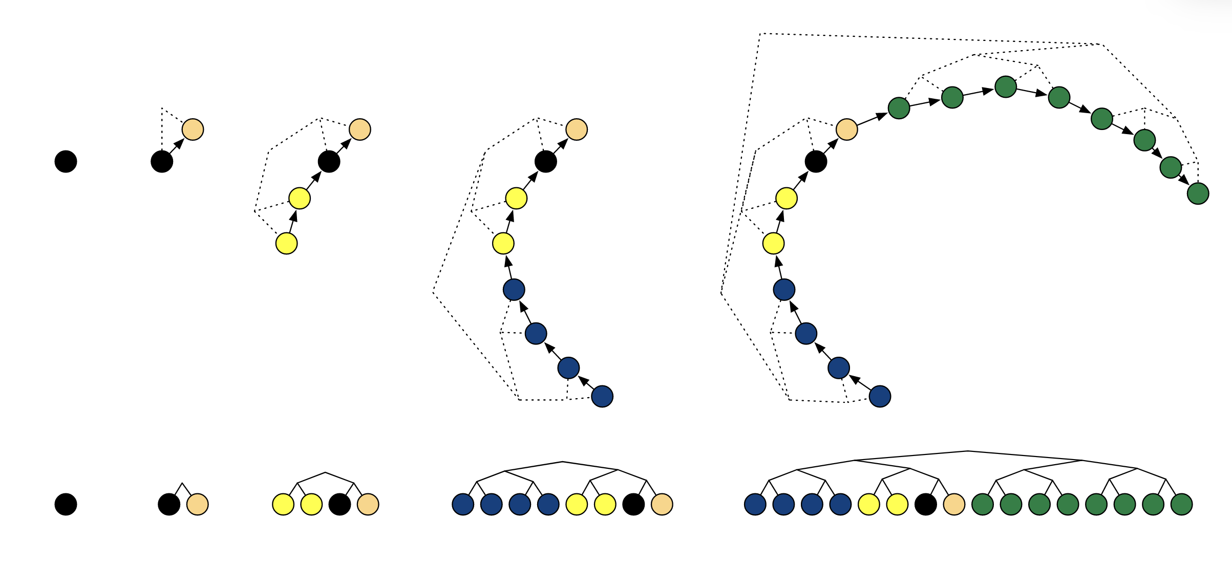
Binary Tree Visualization from Hoffman and Gelman's paper introducing HMC

Figure: The binary tree structure representing the recursive doubling procedure used in HMC-NUTS from the paper "The No-U-Turn Sampler: Adaptively Setting Path Lengths in Hamiltonian Monte Carlo" by Hoffman and Gelman (2011). The caption reads -"Example of building a binary tree via repeated doubling. Each doubling proceeds by choosing a direction (forwards or backwards in time) uniformly at random, then simulating Hamiltonian dynamics for 2j leapfrog steps in that direction, where j is the number of previous doublings (and the height of the binary tree). The figures at top show a trajectory in two dimensions (with corresponding binary tree in dashed lines) as it evolves over four doublings, and the figures below show the evolution of the binary tree. In this example, the directions chosen were forward (light orange node), backward (yellow nodes), backward (blue nodes), and forward (green nodes)."

And maybe in slightly different terms: We expand out from our initial proposal in opposite directions (via Hamiltonian dynamical leaps), randomly picking which one for any given iteration of a doubling procedure we we sucessively take more and more steps in a given doubling until our algorithm tells us to stop. We then find that the adjusted algorithm after some checks⁷ is shown below:

Naive No-U-Turn Sampler (NUTS) Algorithm

Initialise:

Have a target log-density you want to sample from $U(\theta) = \log p(\theta \vert S)$.

Manually choose a starting point $\theta_0$.

Pick a step size $\epsilon \in \mathbb{R}^+$.

Pick the number of samples to generate $K$.

Define a threshold $\Delta_{max}$ (‘typically’ $1000$) to identify Divergences.

Sample: For each iteration $k$ from $1$ to $K$:

Resample momentum: Draw $r_0 \sim \mathcal{N}(0, I)$.

Slice sampling: Draw $u \sim \text{Uniform}\left(0, \exp\{U(\theta_{k-1}) - \frac{1}{2} r_0 \cdot r_0\}\right)$.

Initialise Tree:

Set $\theta^- = \theta-{k-1}, \theta^+ = \theta_{k-1}, r^- = r_0, r^+ = r_0, j = 0$.

Initialise the set of candidate states $C = \{(\theta-{k-1}, r_0)\}$.

Set the stop-criterion indicator $s = 1$.

Recursive Tree Building: While $s = 1$:

Choose a direction $v_j \sim \text{Uniform}(\{-1, 1\})$.

If $v_j = -1$:
\[\theta^-, r^-, \_, \_, C', s' \leftarrow \text{BuildTree}(\theta^-, r^-, u, v_j, j, \epsilon)\]

Else:
\[\_, \_, \theta^+, r^+, C', s' \leftarrow \text{BuildTree}(\theta^+, r^+, u, v_j, j, \epsilon)\]

If $s' = 1$, then update candidates: $C \leftarrow C \cup C'$.

Update stop criterion based on the No-U-Turn condition:$s \leftarrow s' \cdot \mathbb{I}[(\theta^+ - \theta^-) \cdot r^- \ge 0] \cdot \mathbb{I}[(\theta^+ - \theta^-) \cdot r^+ \ge 0]$

$j \leftarrow j + 1$.

Transition: Sample $\theta_k$ uniformly at random from the set of valid states $C$.

BuildTree Function

Takes in $\theta$, $r$, $u$, $v$, $j$, and $\epsilon$:

Base Case ($j = 0$):

Take one leapfrog step in direction $v$: $\theta', r' \leftarrow \text{Leapfrog}(\theta, r, v\epsilon)$.

Define the set $C'$ as $\{(\theta', r')\}$ if $u \le \exp\{\mathcal{L}(\theta') - \frac{1}{2} r' \cdot r'\}$, otherwise $C' = \emptyset$.

Set $s' = \mathbb{I}[u < \exp\{\Delta_{max} + \mathcal{L}(\theta') - \frac{1}{2} r' \cdot r'\}]$.

Return $\theta', r', \theta', r', C', s'$.

Recursion ($j > 0$):

Build the first subtree: $\theta^-, r^-, \theta^+, r^+, C', s' \leftarrow \text{BuildTree}(\theta, r, u, v, j-1, \epsilon)$.

If $s' = 1$:

If $v = -1$:
\[\theta^-, r^-, \_, \_, C'', s'' \leftarrow \text{BuildTree}(\theta^-, r^-, u, v, j-1, \epsilon)\]

Else:
\[\_, \_, \theta^+, r^+, C'', s'' \leftarrow \text{BuildTree}(\theta^+, r^+, u, v, j-1, \epsilon)\]

Update stop criterion: $s' \leftarrow s'' \cdot \mathbb{I}[(\theta^+ - \theta^-) \cdot r^- \ge 0] \cdot \mathbb{I}[(\theta^+ - \theta^-) \cdot r^+ \ge 0]$

Update candidates: $C' \leftarrow C' \cup C''$.

Return $\theta^-, r^-, \theta^+, r^+, C', s'$.

Some things to note:

We have set the mass matrix to the identity (not necessarily indicative of the method but is a pain to write so I won’t include it from now on)
The method makes use of Slice sampling (with the slice variable being $u$)
The tree continues to be constructed until either the sampler starts retracing steps (satisfying the scalar product condition which is quantified by indicator functions e.g. $\mathbb{I}[(\theta^+ - \theta^-) \cdot r^- \ge 0]$) or one of the trajectories has ventured into a very low probability area
We now no longer simply take the last sample in the HMC trajectory but rather uniformly sample from the constructed set $C$ which holds all the points in the trajectory if it contains valid slice sampling proposals i.e. the condition $u \le \exp\{\mathcal{L}(\theta') - \frac{1}{2} r' \cdot r'\}$

Now again, seems great, but the algorithm requires $2^j-1$ evaluations of $\mathcal{L}(\theta)$ and its gradient (where $j$ is the number of times BuildTree() is called), and $\mathcal{O}(2^j)$ additional operations to determine when to stop doubling and it requires us to store $2^j$ position and momentum coordinates … this is not great. But for a simple problem such as a gaussian we can implement this idea fine, this is shown in the GIF below.

Don’t be naive: Updating the transition kernel to make NUTS more efficient

We want to reduce the computational cost incurred above, but there are also better transition kernels and other improvements we can make.

Other kenels can make larger jumps on $C$ so we can explore the probability space more efficiently compared to uniform sampling and sidestep to store all $\mathcal{O}(2^j)$ elements of the full set $C$ which is currently required to uniformly sample it.

We can reduce some waste in the construction of $C'$, because even if $s' = 0$ in the middle of a given iteration of doubling, we continue that given iteration anyways despite there being no point, as proposals after that point will not be used/are wasted samples. I should have addressed this in the first algorithm, just requires checking the condition and exiting during the relevant part of the procedure, but I’m also kinda following the order that Hoffman and Gelman did for their paper and I don’t want to accidentally skip something important.

To fix the issue of storing so many coodinates Hoffman and Gelman suggest the using the following probability ‘quirk’ and transition kernel, which means that instead of having to store $\mathcal{O}(2^j)$, we only have to store $\mathcal{O}(j)$ (or even $\mathcal{O}(1)$).

A relatively straight forward fact is that the probability of selecting any given sample from the whole tree is the product of picking the given depth (number of samples generated at that given depth over the total number of samples), and the probability of picking a given sample from that doubling iteration (1 over the number of samples generated at that given depth).

\[\begin{align} & p(\text{picking $(\theta, r)$ from iteration j from C}) = \frac{1}{\text{total number of samples}} \\ &= \frac{\text{number of samples generated at depth j}}{\text{total number of samples}} \cdot \frac{1}{\text{number of samples generated at depth j}} \\ p(\theta, r| C') &= \frac{1}{\vert C' \vert} = \frac{\vert C_{\text{subtree}} \vert}{\vert C' \vert} \cdot \frac{1}{\vert C_{\text{subtree}} \vert} \\ &=p((\theta, r) \in C_{\text{subtree}}|C) \cdot p(\theta, r|(\theta, r) \in C_{\text{subtree}}, C) \end{align}\]

This allows us to build the tree recursively and not have to store the whole set $C$. i.e. we can sample uniformly from a given doubling iteration and just retain a single sample for use in the wider algorithm, so for $j$ iterations we only need to store $j$ samples!

We can also leverage a better kernel that will bias the sampling to pick samples further along in the chain of doubling iterations (i.e. more likely to sample depth 3 than depth 1 doubling iteration) i.e. whether to move the ‘state’ of the algorithm to this new subtree’s candidate/use the representative sample from previous iterations or the new one.

\[\begin{align} T(z'\vert z, C) = \begin{cases} \frac{\mathbb{I}[z' \in C^{new}]}{\vert C^{new}\vert} & \textrm{if} \vert C^{new}\vert > \vert C^{old}\vert \\ \frac{\vert C^{new}\vert}{\vert C^{old}\vert} \frac{\mathbb{I}[z' \in C^{new}]}{\vert C^{new}\vert} + \left(1 - \frac{\vert C^{new}\vert}{\vert C^{old}\vert} \right) \mathbb{I}[z'=z] & \textrm{if} \vert C^{new}\vert \leq \vert C^{old}\vert \\ \end{cases} \end{align}\]

With $C^{new}$ being samples from the last round of doubling (basically the latest $C_\text{subtree}$ from above), and $C^{old}$ being all the other samples (i.e. $C/C^{new}$) what this kernel is quantifying is the probability of moving from a coordinate $z=(\theta, r) \in C^{old}$ to $z'=(\theta', r') \in C^{new}$.

In practice, we only need to keep track of the current state $(\theta, r)$, the candidate from the new subtree $(\theta', r')$, and the endpoints of the trajectory to check the No-U-Turn condition. With the above improvements we get the following algorithm.

Efficient No-U-Turn Sampler (NUTS) Algorithm

Initialise:

Have a target log-density you want to sample from $U(\theta\vert S) = \log p(\theta \vert S)$.

Manually choose a starting point $\theta_0$.

Pick a step size $\epsilon \in \mathbb{R}^+$.

Pick the number of samples to generate $K$.

Define a threshold $\Delta_{max}$ (typically $\sim 1000$) to identify Divergences.

Sample: For each iteration $l$ from $1$ to $K$:

Resample momentum: Draw $r_0 \sim \mathcal{N}(0, I)$.

Slice sampling: Draw $u \sim \text{Uniform}\left(0, \exp\{U(\theta_{k-1}) - \frac{1}{2} r_0 \cdot r_0\}\right)$.

Initialise Tree:

Set $\theta^- = \theta_{k-1}, \theta^+ = \theta_{k-1}, r^- = r_0, r^+ = r_0, j = 0$.

Set the current sample state $\theta_k = \theta_{k-1}$.

Set the initial count of valid states $n = 1$ and stop-criterion indicator $s = 1$.

Recursive Tree Building: While $s = 1$:

Choose a direction $v_j \sim \text{Uniform}(\{-1, 1\})$.

If $v_j = -1$:
$\theta^-, r^-, \_, \_, \theta', n', s'$ $\leftarrow$ $\text{BuildTree}(\theta^-, r^-, u, v_j, j, \epsilon)$

Else:
$\_, \_, \theta^+, r^+, \theta', n', s'$ $\leftarrow$ $\text{BuildTree}(\theta^+, r^+, u, v_j, j, \epsilon)$

Transition Step: If $s' = 1$, update the sample state with probability $\min\left(1, \frac{n'}{n}\right)$:
$\theta_k$ $\leftarrow$ $\theta'$

Update Counters: $n$ $\leftarrow$ $n + n'$.

Stop Criterion: Update $s$ based on the trajectory endpoints:
$s$ \leftarrow $s' \cdot \mathbb{I}[(\theta^+ - \theta^-) \cdot r^- \ge 0] \cdot \mathbb{I}[(\theta^+ - \theta^-) \cdot r^+ \ge 0]$

$j \leftarrow j + 1$.

BuildTree Function

Takes in $\theta, r, u, v, j, \epsilon$:

Base Case ($j = 0$):

Take one leapfrog step in direction $v$: $\theta', r' \leftarrow \text{Leapfrog}(\theta, r, v\epsilon)$.

Set $n' = \mathbb{I}[u \le \exp\{\mathcal{L}(\theta') - \frac{1}{2} r' \cdot r'\}]$.

Set $s' = \mathbb{I}[u < \exp\{\Delta_{max} + \mathcal{L}(\theta') - \frac{1}{2} r' \cdot r'\}]$.

Return $\theta', r', \theta', r', \theta', n', s'$.

Recursion ($j > 0$):

Build first subtree: $\theta^-, r^-, \theta^+, r^+, \theta', n', s' \leftarrow \text{BuildTree}(\theta, r, u, v, j-1, \epsilon)$.

If $s' = 1$:

Build second subtree:

If $v = -1$:
\[\theta^-, r^-, \_, \_, \theta'', n'', s'' \leftarrow \text{BuildTree}(\theta^-, r^-, u, v, j-1, \epsilon)\]

Else:
\[\_, \_, \theta^+, r^+, \theta'', n'', s'' \leftarrow \text{BuildTree}(\theta^+, r^+, u, v, j-1, \epsilon)\]

Progressive Sampling: With probability $\frac{n''}{n' + n''}$, set $\theta' \leftarrow \theta''$.

Update Stop Criterion:
\[s' \leftarrow s'' \cdot \mathbb{I}[(\theta^+ - \theta^-) \cdot r^- \ge 0] \cdot \mathbb{I}[(\theta^+ - \theta^-) \cdot r^+ \ge 0]\]

Update Count: $n' \leftarrow n' + n''$.

Return $\theta^-, r^-, \theta^+, r^+, \theta', n', s'$.

Translating the mathematical transition kernel definition to it’s practical implementation

To me it wasn’t obvious how the transition kernel defined above translated into the algorithm and so I’m going to dedicate this quick subsection to that. If you’re fine with the above gist then skip this one.

The transition kernel $T(z' \vert z, C)$ defines the probability that we end up at a specific point $z'$ given we started at point $z$.

To see how Algorithm 3 implements this, we have to look at the two different levels where randomness enters the process.

Stage 1: The Representative Selection (Inside BuildTree)

Before the main loop even considers moving, BuildTree must find a “representative” candidate from the new territory. Because we want to sample uniformly from all valid points, the probability that any specific point $z' \in C_{new}$ is chosen as the representative $\theta'$ must be: $P(\theta' = z') = \frac{1}{\vert C_{new}\vert} = \frac{1}{n'}$. This is handled by that “quirky” recursive line:

With probability $n'' / (n' + n'')$, set $\theta' = \theta''$.

This ensures that no matter how many doublings occur, the $\theta'$ that returns to the main loop is a fair representative of its subtree.

Stage 2: The Metropolis-Style Jump (In the Main Loop)

Once BuildTree returns the representative $\theta'$, the main loop decides whether to move the chain there or stay put. This is the $\min(1, n'/n)$ step.The total probability of the algorithm ending up at a specific point $w'$ is the product of these two stages:

\[P(\text{Final state} = w') = P(\text{Selection}) \times P(\text{Acceptance})\]

The Case-by-Case Breakdown

With this we can examine each case in the definition of the transition kernel.

Case 1: The new subtree is larger ($n' > n$)

The kernel says the probability should be $1/n'$.

Selection: $\theta'$ is picked with probability $1/n'$.
Acceptance: $\min(1, n'/n) = 1$.
Total: $(1/n') \times 1 = \mathbf{1/n'}$.

(Matches!)

Case 2: The new subtree is smaller ($n' \le n$)

The kernel says the probability should be $1/n$.

Selection: $\theta'$ is picked with probability $1/n'$.
Acceptance: $\min(1, n'/n) = n'/n$.
Total: $(1/n') \times (n'/n) = \mathbf{1/n}$.

(Matches!)

Final Implementation demonstration

Let’s revisit our NUTS implementation GIF one last time showing how the tree is now utilised in the algorithm. The full trees will still be shown, but keep in mind that the greyed out samples are not stored and basically the act of not having to store and sample over all of them is where most of the efficiency gain is coming from. The samples in the top left are left fully coloured just to show the path, but as above, it’s the same tree as below and the greyed out samples would have been thrown away for efficient computation.

I must be NUTS: Adaptive tuning for $\epsilon$

I was going to do this but I’m already well outside the scope of what I was planning to do with the HMC portion of this post so I’d just recommend having a look at the section “Adaptively Tunring $\epsilon$” in Hoffman and Gelman for this. If you are reading this and really want me to cover it shoot me an email at “[firstname]c[lastname]@[google address].com”.

Overdamped LMC in detail

Langevin Monte Carlo is the algorithmic realization of a specific Stochastic Differential Equation.

While HMC simulates a frictionless orbit, LMC simulates a particle in a high-viscosity fluid.

The Overdamped Langevin SDE

We start with the Overdamped Langevin Equation. Using the notation from our SDE introduction, we set the drift $b(y(t))$ and the diffusion $B(y(t))$ as follows:

\[\begin{equation} dY_t = \underbrace{-\nabla U(Y_t) dt}_{\text{Drift}} + \underbrace{\sqrt{2} dW_t}_{\text{Diffusion}} \end{equation}\]

Here, $U(x) = -\log \pi(x\vert S)$ is still our potential energy (negative log-target).

The constant $\sqrt{2}$ isn’t arbitrary; it is the specific scaling required to ensure the stationary distribution of this process is exactly our target $\pi(x\vert S)$.

Proving the Stationary Distribution via Fokker-Planck

To see why this SDE “samples” our target, we look at the evolution of the probability density $p(x, t)$ using the Fokker-Planck Equation you saw earlier.

For the SDE above, the PDE is:

\[\frac{\partial p(x, t)}{\partial t} = \nabla \cdot \left( p(x, t) \nabla U(x) \right) + \Delta p(x, t)\]

Where $\Delta$ is the Laplacian ($\nabla^2$). For the system to be at equilibrium, the density must stop changing, meaning $\frac{\partial p}{\partial t} = 0$. This occurs when the Probability Flux $J$ is zero.

Let’s test if our target $\pi(x\vert S) \propto e^{-U(x)}$ satisfies this:

Substitute $\pi(x)$ into the flux equation: $J = \pi(x) \nabla U(x) + \nabla \pi(x)$.
Calculate the gradient: $\nabla \pi(x) = \nabla(e^{-U(x)}) = -e^{-U(x)} \nabla U(x) = -\pi(x) \nabla U(x)$.
Plug it back in: $J = \pi(x) \nabla U(x) - \pi(x) \nabla U(x) = 0$.

Because the flux is zero, the distribution is stationary. Physically, the “push” toward the mode (drift) is exactly canceled out by the “spread” of the Brownian motion (diffusion).

Detailed Balance and Ergodicity

In the continuous-time SDE world, the condition $J=0$ is equivalent to Detailed Balance. It implies that the probability of the particle moving from $x \to x'$ is the same as $x' \to x$.

Ergodicity: The Noise Guarantee

Why is LMC ergodic? Irreducibility.

Because the Wiener process $dW_t$ has Gaussian increments, there is a non-zero probability of jumping anywhere in $\mathbb{R}^n$ at any time step.

Unlike a deterministic ODE which can get trapped in a local basin, the stochastic “shocks” ensure the particle can eventually climb any energy barrier $U(x)$, provided the gradient doesn’t explode to infinity.

The Discretization Gap: Enter MALA

On a computer, we cannot solve the SDE exactly. We use the Euler-Maruyama discretization with step size $\epsilon$:

\[\theta_{n+1} = \theta_n - \epsilon \nabla U(\theta_n) + \sqrt{2\epsilon} \xi_n, \quad \xi_n \sim \mathcal{N}(0, I)\]

This is the Unadjusted Langevin Algorithm (ULA), and it is broken and doesn’t do what we want it to do. In our SDE introduction, we noted that $dW \approx \sqrt{dt}$. In discrete steps, this linear approximation of a non-linear gradient introduces a Discretization Error.

Specifically, ULA does not satisfy detailed balance for a finite $\epsilon$. The “drift” pushes the particle slightly further than the continuous path would, leading to a biased stationary distribution $\pi_{\epsilon}(x) \neq \pi(x)$.

With a little more detail, recall the condition:

\[\pi(x) q(x'|x) = \pi(x') q(x|x')\]

In ULA, the transition kernel $q(x'\vert x)$ is the density of the Gaussian proposal:

\[q(x'|x) = \frac{1}{(4\pi\epsilon)^{d/2}} \exp\left( -\frac{\|x' - x + \epsilon \nabla U(x)\|^2}{4\epsilon} \right).\]

Note that $q(\theta' \vert \theta) \neq q(\theta \vert \theta')$. Because the gradient at the start point $\theta$ is different from the gradient at the end point $\theta'$, the proposal is asymmetric.

If we look at the log-ratio of the forward and backward probabilities (which should be zero for symmetry/balance), we get:

\[\log \left( \frac{\pi(x') q(x|x')}{\pi(x) q(x'|x)} \right) = \log \frac{\pi(x')}{\pi(x)} + \log \frac{q(x|x')}{q(x'|x)}\]

Substituting our potential $U(x) = -\log \pi(x)$ and the Gaussian $q$:

\[\dots = [U(x) - U(x')] + \frac{1}{4\epsilon} \left( \|x' - x + \epsilon \nabla U(x)\|^2 - \|x - x' + \epsilon \nabla U(x')\|^2 \right)\]

Expanding the squared norms:

\[\|x' - x + \epsilon \nabla U(x)\|^2 = \|x' - x\|^2 + 2\epsilon(x' - x) \cdot \nabla U(x) + \epsilon^2 \|\nabla U(x)\|^2\]

When you subtract the backward norm from the forward norm, the $\|x' - x\|^2$ terms cancel, but we are left with:

\[\frac{1}{2} (x' - x) \cdot (\nabla U(x) + \nabla U(x')) + \frac{\epsilon}{4} (\|\nabla U(x)\|^2 - \|\nabla U(x')\|^2)\]

Now, compare this to the first-order Taylor expansion of the potential difference $U(x) - U(x')$. If $U$ is smooth, then:

\[U(x) - U(x') \approx \frac{1}{2} (x - x') \cdot (\nabla U(x) + \nabla U(x'))\]

Oops, we shouldn’t have anything of order $\mathcal{O}(\epsilon)$ ($(x - x')$) (or below $\mathcal{O}(1)$, which we thankfully do not have) left around. Meaning that the ULA transition generates an extra term of order $\mathcal{O}(\epsilon)$ that doesn’t exist in the target distribution’s geometry.

Specifically, the $\frac{\epsilon}{4} \|\nabla U\|^2$ terms and the higher-order remainders of the Taylor expansion don’t cancel out unless $\epsilon \to 0$, so if $\epsilon$ is finite, then we have a finite bias.

i.e. Because this ratio is not exactly $1$ (or the log-ratio isn’t $0$), the chain doesn’t converge to $\pi(x)$. It converges to a biased distribution $\pi_\epsilon(x)$ that is “stretched” by the gradient’s local curvature.

To fix this (discretization) gap, we treat the ULA update as a Metropolis-Hastings proposal. This gives us the Metropolis-Adjusted Langevin Algorithm (MALA).

With the same transition kernel (the probability of proposing $\theta'$ from $\theta$) shown again below:

\[q(\theta' \vert \theta) \propto \exp \left( -\frac{1}{4\epsilon} \| \theta' - (\theta - \epsilon \nabla U(\theta) )\|^2 \right),\]

which is basically the usual Metropolis-Hasting’s ‘kinda’ kernel with a symmetric gaussian, except the point that the gaussian is centred on isn’t the previous proposal, but the previous proposal minus the gradient! i.e. We’re more likely to sample higher probability regions.

To satisfy detailed balance in the Markov Chain, we apply the acceptance ratio:

\[\alpha = \min \left( 1, \frac{\pi(\theta') q(\theta | \theta')}{\pi(\theta) q(\theta' | \theta)} \right)\]

This MH step “prunes” the errors introduced by the Euler-Maruyama discretization, ensuring that the chain converges to the exact target $\pi(x\vert S)$ regardless of the step size (though a large $\epsilon$ will still lead to many rejections).

And that’s all you need to make the Overdamped Langevin MC algorithm!

Metropolis-Adjusted Langevin Algorithm

Initialise:

Have a target density you want to sample from $f(x)$ (known up to a normalising constant),

Define the potential energy as the negative log-density: $U(x) = - \log f(x)$,

Manually choose a starting point $x_0$,

Pick a step size $\epsilon > 0$,

Pick the number of samples to generate $N$.

For each iteration $n$ / Repeat $N$ times:

Langevin proposal steps:

Compute the gradient of the log-density at the current state: $\nabla \log f(x_n)$

Generate a proposal point $x^*$ using a drift term plus noise: $x^* = x_n + \frac{\epsilon}{2} \nabla \log f(x_n) + \sqrt{\epsilon} \eta$ where $\eta \sim \mathcal{N}(0, I)$

Metropolis Hastings correction steps:

Compute the proposal densities: $q(x^* \mid x_n) = \mathcal{N}\left(x^* ; x_n + \frac{\epsilon}{2} \nabla \log f(x_n),\epsilon I\right)$ $q(x_n \mid x^*) = \mathcal{N}\left(x_n ; x^* + \frac{\epsilon}{2} \nabla \log f(x^*),\epsilon I\right)$

Compute the acceptance probability: $\alpha = \min\left(1, \frac{f(x^*) q(x_n \mid x^*)}{f(x_n) q(x^* \mid x_n)}\right)$

Draw a random number $u \sim \text{Uniform}(0, 1)$

Accept or reject:

If $u \le \alpha$, set $x_{n+1} = x^*$

If $u > \alpha$, set $x_{n+1} = x_n$

An example of this algorithm in action is shown in the GIF below.

Underdamped Langevin MCMC

A fun and more commonly used Langevin Dynamical MCMC algorithm is Underdamped Langevin MCMC which is basically where you consider the particles to have mass/momentum or if HMC and overdamped LMC had a baby.

Previously, the SDE for _over_damped LMC was,

\[\begin{equation} \text{Overdamped Langevin SDE} := dY_t = \underbrace{-\nabla U(Y_t) dt}_{\text{Drift}} + \underbrace{\sqrt{2} \, dW_t}_{\text{Diffusion}}, \end{equation}\]

the SDE of _under_damped LMC is (jumping straight into the sample notation like in HMC),

\[\begin{equation} \text{Underdamped Langevin SDE} := \begin{cases} d\theta_t = r_t dt & \\ dr_t = -\underbrace{\nabla U(\theta_t) dt}_{\text{Drift}} - \underbrace{r_t dt}_{\text{Friction}} + \underbrace{\sqrt{2} \, dW_t}_{\text{Diffusion}} & \end{cases} \end{equation}\]

which is extremely similar to before but now we’ve split the SDE into a momentum like update (for $d\theta_t$) and a second order update (for $dr_t$) where we additionally consider a “friction” term. This has the stationary distribution of $p(\theta, r) \propto \exp[ -U(\theta) - \frac{1}{2} r^T r]$ (same as before).

But this also looks similar to something else … the HMC updates! We can rewrite them (with unit mass) as below.

\[\begin{equation} \text{HMC Update Rule} := \begin{cases} d\theta_t = r_t dt & \\ dr_t = - \nabla U(\theta_t) dt - r_t dt & \end{cases} \end{equation}\]

i.e. You can view HMC (updates at least) as the boring SDE case of underdamped LMC where the noise has 0 standard deviation / doesn’t exist.

(The similarity between these almost makes one think there might be some unified way to express these kinds of gradient boosted MCMC algorithms?? If uninterested in underdamped LMC, jump straight to Recipes for Stochastic Gradient MCMC)

Although I’m lying to you a little bit⁸. The more general form of underdamped LMC also includes a friction coefficient that looks like this,

\[\begin{align} \text{Underdamped Langevin SDE}':= \begin{cases} d\theta_t = r_t dt & \\ dr_t = -\underbrace{\nabla U(\theta_t) dt}_{\text{Drift}} - \underbrace{\gamma r_t dt}_{\text{Friction}} + \underbrace{\sqrt{2\gamma} \, dW_t}_{\text{Diffusion}} & \end{cases}. \end{align}\]

For the following I’ll following/yoinking some results from “Underdamped Langevin MCMC: A non-asymptotic analysis” - Xiang Cheng et al. (2018).

The solution to the above (with initial condition $(\theta_0, r_0)$) can be expressed as,

\[\begin{align} \theta_t &= \theta_0 + \int_0^t r_s ds, \\ r_t &= r_0 \exp(-\gamma t) - \left(\int_0^t \exp(-\gamma (t - s)) \nabla \log f(\theta_0) ds \right) + \sqrt{2\gamma} \int_0^t \exp(-\gamma (t - s)) dW_s. \end{align}\]

We can see that the initial conditions are obviously satisfied. But to verify the rest of the solution (which in the paper is left to the reader…), we take the time derivative of $r_t$ using the Leibniz Integral Rule (for the deterministic part) and Itô’s Lemma (for the stochastic part).

\[\begin{align} dr_t &= d(r_0 e^{-\gamma t}) + d\left( \int_0^t e^{-\gamma(t-s)} \nabla \log f ds \right) + d\left( \sqrt{2\gamma} \int_0^t e^{-\gamma(t-s)} dW_s \right) \\ &= -\gamma r_0 e^{-\gamma t} dt \\ &\;\;\;\;\; + \nabla \log f(\theta_t) dt - \gamma \left( \int_0^t e^{-\gamma(t-s)} \nabla \log f ds \right) dt \\ &\;\;\;\;\; + \sqrt{2\gamma} dW_t - \gamma \left( \sqrt{2\gamma} \int_0^t e^{-\gamma(t-s)} dW_s \right) dt \\ &= -\gamma \left( r_0 e^{-\gamma t} - \left( \int_0^t e^{-\gamma(t-s)} \nabla \log f ds \right) + \sqrt{2\gamma} \int_0^t e^{-\gamma(t-s)} dW_s \right) dt \\ &\;\;\;\;\; + \nabla \log f(\theta_t) dt + \sqrt{2\gamma} dW_t \\ &= - \gamma r_t dt -\nabla U(\theta_t) dt + \sqrt{2\gamma} \, dW_t \end{align}\]

Because the Wiener process $dW_s$ is Gaussian, any linear operation on it (like our integration) results in a Gaussian distribution.

Thus for discrete time steps (the discrete-time Markov process rather than the continuous time), the transition from step $t$ to $t+\delta$ is a multivariate Gaussian. Assuming $\nabla \log f(\theta_t)$ is constant over the small interval $\delta$, the exact solution yields the following expectations:

\[\begin{align} \mathbb{E}[\theta_{t+\delta}] &= \theta_t + \frac{1}{\gamma}(1-e^{-\gamma \delta}) r_t + \frac{1}{\gamma} \left( \delta - \frac{1-e^{-\gamma \delta}}{\gamma} \right) \nabla \log f(\theta_t) \\ \mathbb{E}[r_{t+\delta}] &= r_t e^{-\gamma \delta} + \frac{1}{\gamma}(1-e^{-\gamma \delta}) \nabla \log f(\theta_t) \end{align}\]

And the covariances:

\[\begin{align} \text{Cov}[\theta_{t+\delta}] &= \frac{1}{\gamma^2} \left[ 2\gamma \delta - 3 + 4e^{-\gamma \delta} - e^{-2\gamma \delta} \right] \cdot I_d \\ \text{Cov}[r_{t+\delta}] &= [1 - e^{-2\gamma \delta}] \cdot I_d \\ \text{Cov}[\theta_{t+\delta}, r_{t+\delta}] &= \frac{1}{\gamma} [1 - e^{-\gamma \delta}]^2 \cdot I_d \end{align}\]

A more explicit proof is shown for Lemma 11 in Xiang Cheng et al. (2018) although they set $\gamma=2$, so you might have to go back and forth between what I have and what they show to know explicitly what happens to that. This motivates the below algorithm for underdamped Langevin Monte Carlo.

Underdamped Langevin Monte Carlo (ULMC)

Initialise:

Have a target density you want to sample from $f(\theta)$.

Define the gradient of the log-density: $\nabla \log f(\theta)$.

Manually choose a starting position $\theta_0$and initial momentum$r_0 \sim \mathcal{N}(0, I_d)$.

Pick a step size $\delta > 0$ and a friction coefficient $\gamma > 0$.

Pick the number of samples to generate $N$.

For each iteration $t$ in $1$ to $N$:

Compute Deterministic Means:

Compute the current gradient: $g_t = \nabla \log f(\theta_t)$.

Compute expected position: $\mu_{\theta} = \theta_t + \frac{1}{\gamma}(1-e^{-\gamma \delta}) r_t + \frac{1}{\gamma} \left( \delta - \frac{1-e^{-\gamma \delta}}{\gamma} \right) g_t$

Compute expected momentum: $\mu_{r} = r_t e^{-\gamma \delta} + \frac{1}{\gamma}(1-e^{-\gamma \delta}) g_t$

Generate Correlated Noise:

Precompute or use the current variances:

$V_{\theta}$ $=$ $\frac{1}{\gamma^2} [ 2\gamma \delta - 3 + 4e^{-\gamma \delta} - e^{-2\gamma \delta} ]$

$V_{r}$ $=$ $1 - e^{-2\gamma \delta}$

$C_{\theta,r}$ $=$ $\frac{1}{\gamma} [1 - e^{-\gamma \delta}]^2$

Sample two independent vectors $Z_1, Z_2 \sim \mathcal{N}(0, I_d)$.

Transform to correlated noise via Cholesky decomposition:

$r_{noise}$ $=$ $\sqrt{V_{r}} Z_1$

$\theta_{noise}$ $=$ $\frac{C_{\theta,r}}{\sqrt{V_{r}}} Z_1 + \sqrt{V_{\theta} - \frac{C_{\theta,r}^2}{V_{r}}} Z_2$

Update State: Set the next sample and momentum:

$\theta_{t+1}$ $=$ $\mu_{\theta} + \theta_{noise}$

$r_{t+1}$ $=$ $\mu_{r} + r_{noise}$

The algorithm in action can be seen in the below GIF.

Note that it doesn’t have a Metropolis correction step. Oftentimes people run the above with no correction as the biased induced is small enough not to care. If we want the 100% correct solution though we can chuck the metropolis step in which just requires one to figure out the probability of transition from the proposal to the current sample.

Metropolis-Adjusted Underdamped Langevin Algorithm (MAULA)

Initialise:

Have a target density you want to sample from $f(\theta)$.

Define the gradient of the log-density: $\nabla \log f(\theta)$.

Manually choose a starting position $\theta_0$ and initial momentum $r_0 \sim \mathcal{N}(0, I_d)$.

Pick a step size $\delta > 0$ and a friction coefficient $\gamma > 0$.

Pick the number of samples to generate $N$.

For each iteration $t$ in $1$ to $N$:

Compute Deterministic Means:

Compute the current gradient: $g_t = \nabla \log f(\theta_t)$.

Compute expected position: $\mu_{\theta} = \theta_t + \frac{1}{\gamma}(1-e^{-\gamma \delta}) r_t + \frac{1}{\gamma} \left( \delta - \frac{1-e^{-\gamma \delta}}{\gamma} \right) g_t$

Compute expected momentum: $\mu_{r} = r_t e^{-\gamma \delta} + \frac{1}{\gamma}(1-e^{-\gamma \delta}) g_t$

Generate Correlated Noise:

Precompute the variances and covariance:

\[V_{\theta} = \frac{1}{\gamma^2} [ 2\gamma \delta - 3 + 4e^{-\gamma \delta} - e^{-2\gamma \delta} ]\]

\[V_{r} = 1 - e^{-2\gamma \delta}\]

\[C_{\theta,r} = \frac{1}{\gamma} [1 - e^{-\gamma \delta}]^2\]

Sample two independent vectors $Z_1, Z_2 \sim \mathcal{N}(0, I_d)$.

Transform to correlated noise via Cholesky decomposition:

\[r_{\text{noise}} = \sqrt{V_{r}} Z_1\]

\[\theta_{\text{noise}} = \frac{C_{\theta,r}}{\sqrt{V_{r}}} Z_1 + \sqrt{V_{\theta} - \frac{C_{\theta,r}^2}{V_{r}}} Z_2\]

Propose New State:

\[\theta^* = \mu_{\theta} + \theta_{\text{noise}}\]

\[r^* = \mu_{r} + r_{\text{noise}}\]

Compute Reverse Proposal (for detailed balance):

Compute gradient at proposal: $g^* = \nabla \log f(\theta^*)$.

Compute reverse means:

\[\mu_{\theta}^{\text{rev}} = \theta^* + \frac{1}{\gamma}(1-e^{-\gamma \delta}) (-r^*) + \frac{1}{\gamma} \left( \delta - \frac{1-e^{-\gamma \delta}}{\gamma} \right) g^*\]

\[\mu_{r}^{\text{rev}} = (-r^*) e^{-\gamma \delta} + \frac{1}{\gamma}(1-e^{-\gamma \delta}) g^*\]

Compute Acceptance Probability:

Forward proposal density: $q((\theta^*, r^*) \vert (\theta_t, r_t))$

Reverse proposal density: $q((\theta_t, -r_t) \vert (\theta^*, -r^*))$

\[\alpha = \min\left(1, \frac{f(\theta^*) \exp(-\frac{1}{2}\vert r^*\vert^2) \cdot q((\theta_t, -r_t) \vert (\theta^*, -r^*))}{f(\theta_t) \exp(-\frac{1}{2}\vert r_t\vert ^2) \cdot q((\theta^*, r^*) \vert (\theta_t, r_t))}\right)\]

Accept or Reject:

Draw $u \sim \text{Uniform}(0, 1)$

If $u \le \alpha$:

\[\theta_{t+1} = \theta^*\]

\[r_{t+1} = r^*\]

Else:

\[\theta_{t+1} = \theta_t\]

$r_{t+1} = -r_t$ (negate momentum on rejection)

And again, you can see the process in the GIF below, which you can use as a point of comparison for the level of biased induced without the Metropolis step (not a lot.)

One of the key points of difference between our final result here and HMC is that you don’t need to resample the momentum, the noise induced in that step is part of the dynamics. i.e. the process is ergodic without the need to throw in extra resampling. And we don’t need to chop off our traversals, because we don’t have any! But it’s not all solved or anything, we swapped the issue of figuring out the traversal length with figuring out what the friction coefficient $\gamma$ should be.

Recipes for Stochastic Gradient MCMC

One of the (if not the) main drawbacks when it comes to the above is the calculation of the full gradient. i.e. the derivative of the likelihood requires one to analyse all of their data.

But one of the reasons that people fall to these methods is that they are dealing with large datasets, and thus the likelihood and it’s gradient can be quite expensive to compute.

So, what we might want to do is use subsets, or minibatches, of our data during sampling. And for now, and as “A Complete Recipe for Stochastic Gradient MCMC” - Ma et al. do, we’ll focus on the dynamics/the proposals. i.e. Like doing under- or over-damped LMC can kinda be done without the Metropolis correction. We’ll leave someone else to figure out how to nicely do that (but really it should be pretty simple, just do the same thing we did with underdamped LMC but would require an evaluation of the likelihood with the full dataset).

However, there are issues that can pop up when this is done, primarily biased solutions like in “Stochastic gradient Hamiltonian Monte Carlo” (SGHMC) - Chen et al. without the explicit correction they propose.

Ma et al. looks at a generalising descriptions of continuous Markov processes in part to identify legitimate unbiased continuous processes i.e. ones that converge to the correct distribution.

Ma et al. describe the process with the following SDE.

\[\begin{align} dz = f(z) dt + \sqrt{2 D(z)} dW(t) \end{align}\]

Where $f(z)$ is the force driving the process and $\sqrt{2 D(z)}$ is the amplitude of the noise with $D(z)$ being a positive semidefinite diffusion matrix. Like in the SDE update rule for HMC, if $D(z)=0$, the process becomes deterministic. In which case, instead of asking whether the process converges on the distribution (the samples are distributed according to the target distribution), we want the process to leave the distribution invariant.

Invariant here meaning that once the system reaches that distribution, it stays there. i.e. a steady state. If we have a collection of particles distributed according to our target density $p(z \vert S)$, and apply the dynamics described by your SDE (the drift and the diffusion), the overall shape of that distribution doesn’t change over time. And for the ergodicity of the deterministic processes, some sort of jump process has to be added, like the momentum resampling in HMC.

Ma et al. then provide an ansatz for required form of the drift term, such that the process converges on our target density $p(z \vert S)$ or leaves it invariant:

\[\begin{align} f(z) = - [D(z) + Q(z)]\nabla H(z) + \Gamma(z), \end{align}\]

with,

\[\begin{align} \Gamma_i(z) = \sum_{j=1}^d \frac{\partial}{\partial z_j} (D_{ij}(z) + Q_{ij}(z)), \;\;\;\; i \in \{1,2,..., d\}, \end{align}\]

where the target distribution $p_s(\theta)$ is $d$-dimensional. With the Hamiltonian defined similar to above, where $U$ is as defined above, $r$ just represents ‘auxillary’ variables not specifically momentum, and $H(z) = H(\theta, r) = U(\theta) + g(\theta, r)$ with $\int \exp(-g(\theta, r)) dr = \text{const.}$.

This is done such that the distribution $p_s(\theta)$ is proportional to $\int p(z)dr = \int p(\theta, r)dr \propto \int \exp(-H(\theta, r)) dr = \exp(-U(\theta)) \int \exp(-g(\theta, r)) dr \propto p(\theta) \cdot \text{const.}$.

But back to the ansatz, according to it, any continuous markov process with target distribution $p(z)$, is entirely described by two matrices. $Q(z)$, a skew-symmetric curl matrix representing the deterministic traversing effects and $D(z)$, the diffusion matrix, determining the strength of the Wiener process-driven diffusion. According to Ma et al. faster convergence to the posterior distribution can be achieved by adjusting $D(z)$ and $Q(z)$.

The update rule for this setup is:

\[\begin{align} z_{t+1} \leftarrow z_t - \epsilon_t \left[\left(D(z_t) + Q(z_t)\right) \nabla H(z_t) + \Gamma(z_t)\right] + \mathcal{N}(0, 2\epsilon D_t) \end{align}\]

For their claims to be true they need to show two things: 1. That the stationary distribution/stead-state solution to the SDE/update rule, $p_s(z)$, is either equivalent to the target distribution $p(z \vert S)$ or the evolution of the SDE leaves the target distribution invariant. This is shown in theorem 1 in the paper.

Theorem 1

$p_s(z) \propto \exp(−H(z))$ is a stationary distribution of the dynamics of the SDE $dz = f(z) dt + \sqrt{2 D(z)} dW(t)$ if $f(z)$ is restricted to the form [shown above], with $D(z)$ positive semidefinite and $Q(z)$ skew-symmetric. If $D(z)$ is positive definite, or if ergodicity can be shown, then the stationary distribution is unique.

The proof shown for this in the paper is pretty straightforward and I’ll leave you to read it there (otherwise I’d just be copy-pasting). And then they show that every continuous markov process that leaves the target distribution invariant, can be described via their framework ($D$ and $Q$) via the following theorem.

Theorem 2

For the SDE $dz = f(z) dt + \sqrt{2 D(z)} dW(t)$, suppose its stationary probability density function $p_s(z)$ uniquely exists, and that $\left[f_i(z)p_s(z) - \sum_{j=1}^d \frac{\partial}{\partial \theta_j}\left(D_{ij}(z)p_s(z)\right) \right]$ is integrable with respect to the Lebesgue measure, then there exists a skew-symmetric $Q(z)$ such the above expression for $f(z)$ holds.

And I’ll leave the proof this theorem for another dedicated post, as to met at least, it’s quite involved/complicated.

Exploring Methods discussed in Ma et al. (2015) and those above

To cap off the post, I’m going to go through each of the methods mentioned in Ma et al. and those above, specifically: how they translate into the formalism Ma et al. describe, and some GIFs showing how they converge on different targets.

The targets I’ll investigate are a standard 2D normal (as done above), a 2D student-t distribution with unit scale matrix and the Rosenbrock distribution with $a=1$ and $b=2$ as well as the Banana distribution as discussed in “Disentangling impact of capacity, objective, batchsize, estimators, and step-size on flow VI”.

I’ll skip the definitions for the first three distributions (easily google-able).

Banana Distribution

$z_1$ $\sim$ $\mathcal{N}(0, 10^2)$

$z_2$ $\sim$ $\mathcal{N}(0.03(z_1^2 - 100), 1)$

$z_i$ $\sim$ $\mathcal{N}(0, 1)$ $\text{for} \;\; i=3, ..., d$

For the Banana distribution we’ll not include $i\geq 3$. Some examples of what this look using some corner plots is shown below.

HMC

I’m not going to make the GIFS for HMC as they basically amount to gradient descent, but it’s interesting (to me at least) how simple HMC is in the framework proposed.

If our update rule with no stochastic estimates (and neglecting the mass matrix) is:

\[\begin{align} \begin{cases} \theta_{t+1} \leftarrow \theta_t + \epsilon_t r_t & \\ r_{t+1} \leftarrow r_t - \epsilon_t \nabla U(\theta_t) & \\ \end{cases} \end{align}\]

Then $z=(\theta, r)$, $H(\theta, r) = U(\theta) + \frac{1}{2} r^T r$. And then in the framework there isn’t any diffusion in the updates, thus $D(\theta, r) = \vec{0}$ and the curl matrix is $Q(\theta, r) = \begin{pmatrix} 0 & -I \\ I & 0 \end{pmatrix}$. Plugging this into the generalised update rule we find,

Overdamped Langevin Dynamics

Overdamped Langevin Dynamics doesn’t have auxillary variables so $z_t = \theta_t$ and $Q(z_t) = 0$. The update rule (with no stochastic updates), which I’ll put again here so you’re not scrolling back and forth is:

\[\begin{align} \theta_{t+1} \leftarrow \theta_t - \epsilon \nabla U(\theta_t) + \mathcal{N}(0, 2\epsilon D) \end{align}\]

Hence, $D(z_t) = D$ and $\Gamma(z_t) = 0$. A one-to-one can then be made with the generalised update rule. Below are some examples of the kind of dynamics with these matrices.

Underdamped Langevin Dynamics

Underdamped Langevin Dynamics includes momenta auxillary variables like HMC. Again, for ease of reading, here is the update rule for underdamped-langevin dynamics (sans friction coefficient).

\[\begin{align} \begin{cases} \theta_{t+1} \leftarrow \theta_t + \epsilon_t r_t \\ r_{t+1} \leftarrow r_t - \epsilon_t (\nabla U(\theta_t) + r_t) + \mathcal{N}(0, 2\epsilon_t D)\\ \end{cases} \end{align}\]

With the same Hamiltonian as HMC, $D(z_t) = \begin{pmatrix} 0 & 0 \\ 0 & D \end{pmatrix}$, $H(z_t) = \begin{pmatrix} 0 & -I \\ I & I \end{pmatrix}$, $\Gamma(z_t) = 0$. Just checking to see that this matches let’s plug it into the generalised update rule.

\[\begin{align} z_{t+1} = \begin{pmatrix} \theta_{t+1} \\ r_{t+1} \end{pmatrix} &\leftarrow z_t - \epsilon_t \left[(D(z_t) + Q(z_t))\nabla H(z_t) + \Gamma(z_t) \right] + \mathcal{N}(0, 2\epsilon_t D(z_t))\\ &= \begin{pmatrix} \theta_{t} \\ r_{t} \end{pmatrix} - \epsilon_t \left[\left(0 + \begin{pmatrix} 0 & -I \\ I & I \end{pmatrix}\right) \nabla H(z_t) + 0 \right] + \begin{pmatrix} 0 \\ \mathcal{N}(0, 2\epsilon_t D) \end{pmatrix} \\ &= \begin{pmatrix} \theta_{t} \\ r_{t} \end{pmatrix} - \epsilon_t \begin{pmatrix} 0 & -I \\ I & I \end{pmatrix} \begin{pmatrix} \nabla U(\theta_t) \\ r_t \end{pmatrix} + \begin{pmatrix} 0 \\ \mathcal{N}(0, 2\epsilon_t D) \end{pmatrix}\\ &= \begin{pmatrix} \theta_{t} \\ r_{t} \end{pmatrix} + \epsilon_t \begin{pmatrix} r_t \\ -(\nabla U(\theta_t) + r_t) \end{pmatrix} + \begin{pmatrix} 0 \\ \mathcal{N}(0, 2\epsilon_t D) \end{pmatrix}\\ &= \begin{pmatrix} \theta_{t} + \epsilon_t r_t \\ r_{t} - \epsilon_t (\nabla U(\theta_t) + r_t) + \mathcal{N}(0, 2\epsilon_t D)\end{pmatrix}\\ \end{align}\]

Below are some examples of the kind of dynamics with these matrices.

HMC-NUTS

Not related to the paper really because I’m using the NUTS algorithm, but I thought it would be fun to see NUTS on these datasets.

Stochastic Gradient (overdamped) Langevin Dynamics (SGLD)

The update rule and how Stochastic Gradient (overdamped) Langevin Dynamics fits into the framework is basically the same as Overdamped Langevin Dynamics except for the gradient noise estimate $\hat{B}_t$.

Below are some examples of the kind of dynamics with these matrices (presuming $\hat{B}_t=0$ for simplicity).

Stochastic Gradient Hamiltonian Monte Carlo (SGHMC)

Now, if you wanted to use stochastic estimates for the gradients in HMC, that you could kinda just swap them in. Well, as Ma et al. point out, if we just write out the update rule using $\nabla \tilde{U}$ as. our stochastic estimate for $\nabla U$:

\[\begin{align} \begin{cases} \theta_{t+1} \leftarrow \theta_t + \epsilon_t r_t & \\ r_{t+1} \leftarrow r_t - \epsilon_t \nabla \tilde{U}(\theta_t) \approx r_t - \epsilon_t \nabla U(\theta_t) + \mathcal{N}(0, \epsilon_t^2 V(\theta)) \\ \end{cases} \end{align}\]

Where we say $\nabla \tilde{U}(\theta_t) \approx \nabla U(\theta_t) + \mathcal{N}(0, V(\theta))$ to say that our stochastic estimate of the gradient is the true gradient plus some gaussian noise with unknown covariance $V(\theta)$. There is an easy comparison to be made with the generalised update rule, and that the diffusion covariance $V(\theta)$, should also be within the gradient update term.

i.e. the noise added to the updates to the momentum leads us to believe something like $D(z_t) = \begin{pmatrix} 0 & 0 \\ 0 & \epsilon_t V(\theta_t) \end{pmatrix}$, but if we plug this and our $H(z_t)$ and $Q(z_t)$ defined similarly to/the same as before into our generalised update rule and expand we find,

\[\begin{align} z_{t+1} = \begin{pmatrix} \theta_{t+1} \\ r_{t+1} \end{pmatrix} &\leftarrow z_t - \epsilon_t \left[(D(z_t) + Q(z_t))\nabla H(z_t) + \Gamma(z_t) \right] + \mathcal{N}(0, 2\epsilon_t D(z_t))\\ &= \begin{pmatrix} \theta_{t} \\ r_{t} \end{pmatrix} - \epsilon_t \left[\left(\begin{pmatrix} 0 & 0 \\ 0 & \epsilon_t V(\theta_t) \end{pmatrix} + \begin{pmatrix} 0 & -I \\ I & 0 \end{pmatrix}\right) \nabla H(z_t) + 0 \right] + \begin{pmatrix} 0 \\ \mathcal{N}(0, 2\epsilon_t (\epsilon_t V(\theta_t))) \end{pmatrix} \\ &= \begin{pmatrix} \theta_{t} \\ r_{t} \end{pmatrix} - \epsilon_t \begin{pmatrix} 0 & -I \\ I & \epsilon_t V(\theta_t) \end{pmatrix} \begin{pmatrix} \nabla U(\theta_t) \\ r_t \end{pmatrix} + \begin{pmatrix} 0 \\ \mathcal{N}(0, 2\epsilon_t^2 V(\theta_t)) \end{pmatrix}\\ &= \begin{pmatrix} \theta_{t} \\ r_{t} \end{pmatrix} + \epsilon_t \begin{pmatrix} r_t \\ -\nabla U(\theta_t) - \epsilon_t V(\theta_t) r_t \end{pmatrix} + \begin{pmatrix} 0 \\ \mathcal{N}(0, 2\epsilon_t^2 V(\theta_t)) \end{pmatrix}\\ &= \begin{pmatrix} \theta_{t} + \epsilon_t r_t \\ r_{t} - \epsilon_t (\nabla U(\theta_t) + \epsilon_t V(\theta_t) r_t ) + \mathcal{N}(0, 2\epsilon_t^2 V(\theta_t))\end{pmatrix}\\ \end{align}\]

So because the original update rule doesn’t fit into the framework, seeing as the diffusion matrix required for the added noise would have to come through in the gradient updates, we can surmise that the distribution that it would converge on would have to be biased. As any dynamics that converge on the target distribution or leave the target distribution invariant can be represented by the above update rule.

In practice we don’t know what $\epsilon_t V(\theta_t)$ is so it’s more common to use a conservative estimate $C \succ \epsilon V(\theta_t)$ and then a adjustment $\hat{B}_t$ that is an estimate of $V(\theta_t)$ is applied such that the update rule fits in with the generalised SDE for stochastic gradient updates.

\[\begin{align} \begin{cases} \theta_{t+1} \leftarrow \theta_t + \epsilon_t r_t & \\ r_{t+1} \leftarrow r_t - \epsilon_t \nabla \tilde{U}(\theta_t) - \epsilon_t C r_t + \mathcal{N}(0, \epsilon_t (2C - \epsilon_t \hat{B}_t))\\ \end{cases} \end{align}\]

Below are some examples of the kind of dynamics (presuming $\hat{B}_t=0$ for simplicity) with these matrices. Although I should emphasize, that with the noise it kinda looks like SGHMC is sampling the space, it is not, it’s just a noisy optimiser basically. Key point from the above is that the dynamics leave the distribution invariant, they don’t actually converge on the target distribution.

Stochastic Gradient Nosé-Hoover Thermostat (SGNHT)

Never heard of this one before the paper either. I believe Ma et al., besides the fact that it’s pretty cool as a method, wanted to show that ‘auxillary’ variables doesn’t just have to mean momentum.

The method was first formally described “Bayesian Sampling Using Stochastic Gradient Thermostats” - Ding et al. (link is straight to the pdf).

With the possibility of misrepresenting the paper, one of the main motivations behind the introduction of the method is that the $\hat{B}_t$ above, the noise covariance meant to offset the true noise, is hard to estimate and needs to be included for larger step sizes (which I get around partly above by using very small step sizes and knowing the scales of the distributions beforehand).

What one would want, is some dynamical system, that would self adjust and effectively fit the noise without the user explicitly specifying it.

The observation they make is that the above samplers (primarily SGHMC) are inspired by physical systems where the probability of states follows what we call the canonical ensemble meaning that $\rho(\theta, r) \propto \exp\left(-H(\theta, r)/(k_B T) \right)$ where $k_B$ is the Boltzmann constant and $T$ is temperature. So as to not overload you with information (if I haven’t already…), these systems satisfy the following,

\[\begin{align} k_B T = \frac{2}{d} \mathbb{E}[K(r)] = \frac{1}{d} \mathbb{E}[r^T r] \;\;\;\;\; (\text{Thermal Equilibrium Condition}) \end{align}\]

($d$ is the dimension of $\theta$). Typically what is implicitly done is $k_B T = 1$ such that $\rho(\theta, r) \propto \exp\left(-H(\theta, r) \right)$ and $\rho(\theta) \propto \exp\left(-U(\theta) \right)$. To stay physical, the systems have to maintain the thermal equilibrium condition among other reasons.

Ding et al. state that standard HMC and Langevin dynamics satisfy this, but once one introduces stochastic estimates ( the “S” in SGLD, or SGHMC) for what are effectively forces from a physical interpretation, then a poorly estimated $\hat{B}_t$ may lead to this condition being violated.

This motivates Ding et al. to introduce what they call a thermostat denoted $\xi$ which would adaptively control the mean kinetic energy (basically a Lagrange multipler). They introduce the dynamics as a differential equation:

\[\begin{align} &d\theta = r \, dt \\ &dr = -\tilde{f}(\theta) \, dt - \xi \, r \,dt + \sqrt{2A}\mathcal{N}(0, dt) \\ &d\xi = \left(\frac{1}{n} r^T r - 1 \right) \, dt. \\ \end{align}\]

Where $A$ is effectively the same as $C$ above. For actually computing this, the update rule is then:

\[\begin{align} &\theta_{t+1} = \theta_{t} + \epsilon_t r_t \\ &r_{t+1} = r_t - \epsilon_t \nabla \tilde{U}(\theta_t) - \epsilon_t \xi_t \, r_t +\mathcal{N}(0, 2\epsilon_t A) \\ &\xi_{t+1} = \xi_t + \epsilon_t\left(\frac{1}{n} r_t^T r_t - 1 \right) \\ \end{align}\]

Following Ding et al.’s explanation. Intuitively, we see that

if $\frac{1}{n} r_t^T r_t$ is less than 1, $\xi_t$ will decrease and lead to $r_{t+1}$ to being bigger than otherwise (i.e. if $\xi=0$) on the next update.
And vice versa, if $\frac{1}{n} r_t^T r_t$ is larger than 1, $\xi_t$ will increase and lead to $r_{t+1}$ to being smaller than otherwise (if $\xi=0$) on the next update.

So the thermostat follows what Ding et al. claim, and effectively means that the system self corrects. Ain’t that fun! (actually though)

Within the framework in Ma et al. this translates into:

$z$ $=$ $(\theta, r, \xi)$
$H(\theta, r, \xi)$ $=$ $U(\theta) + \frac{1}{2}r^T r + \frac{1}{2d}(\xi - D)^2$
$D(\theta, r, \xi)$ $=$ $\begin{pmatrix} 0 & 0 & 0 \\ 0 & A \cdot I & 0 \\ 0 & 0 & 0\end{pmatrix}$
$Q(\theta, r, \xi)$ $=$ $\begin{pmatrix} 0 & -I & 0 \\ I & 0 & r/d \\ 0 & -r^T/d & 0\end{pmatrix}$

Below are some examples of the kind of dynamics with these matrices including the thermostat $\xi$ and the effective temperature $\frac{1}{d} r^T r$. Like SGHMC though, this method is meant to be deterministic, the stochastic nature is purely from the stochastic estimates of the gradient. It’s actually pretty informative to compare the GIFs between SGHMC and SGNHT, as SGNHT is essentially a stabilised version of SGHMC. This stability is extremely evident when you compare the GIFs for the Rosenbrock distribution.

Stochastic Gradient Riemann Hamiltonian Monte Carlo

This method was actually first proposed by Ma et al. in their paper with the help of the proposed framework.

The basic motivation is similar to/the same as for Stochastic Gradient Langevin Dynamics (which I’ll describe next) where we want to give information about the curvature of the distribution being traversed to the framework. Leaving the Hamiltonian alone, they modify $D$ and $Q$ as

$D(\theta, r)$ $=$ $\begin{pmatrix} 0 & 0 \\ 0 & G(\theta)^{-1} \end{pmatrix}$,
$Q(\theta, r)$ $=$ $\begin{pmatrix} 0 & G(\theta)^{-1/2} \\ G(\theta)^{-1/2} & 0 \end{pmatrix}$.

What this basically amount to is that when the likelihood has high curvature, $G(\theta)>>1$, then we add less diffusion via $G(\theta)^{-1}<<1$, and generally thus $G(\theta)^{-1/2}<<1$, and take generally smaller steps.

This also holds for any positive semi-definite $G(\theta)$ which they called generalized SGRHMC which can be useful is the Fisher info is hard to calculate.

Again with $\hat{B}_t=0$, we can observe the dynamics of this below. I’ve also included an ellipse which is spanned by the eigenvectors for $G(\theta)$ which magnitude $G(\theta)^{-1/2}<<1$. Notably, it’s still inherently deterministic with noise coming from the stochastic gradient updates, so again, it’s more like an overcomplicated optimiser, without the momentum resampling.

Stochastic Gradient Riemannian (overdamped) Langevin Dynamics (SGRLD)

SGRLD can be understood as a generalisation of SGLD where the diffusion matrix adapts to the local curvature via the Fisher information matrix $D(\theta)=G^{-1}(\theta)$ but because $D(\theta)$ also comes through in the gradient updates of $\nabla H(\theta)$ it can also be thought to adaptively adjust the step size based on the curvature as well!

Still with $Q(\theta)=\hat{B}_t=0$ the dynamics looks like those below, with the same ellipse as above.

Conclusion

And that’s that. Hope you found the post interesting and useful. In another work I may or may not develop more on Langevin Monte Carlo samplers, particularly “Fluctuation without dissipation: Microcanonical Langevin Monte Carlo” by Robnik and Seljak, that in (a very small) part use the framework introduced by Ma et al. to construct their sampler.

← Previous post

But what are Gibbs and slice sampling?

Footnotes

If you can get around it, I’d love to talk to you about future investment opportunities with the boatloads of money you’d make. ↩
I vehemently detest dot notation, despite most of the literature around this using it, I refuse. ↩
Wiener named after Norbert Wiener is pronounced with a “v” but that doesn’t stop me 100% reading as a “w” to make the papers I read funnier, and yes, I am a child. ↩
The Stratonovich Integral is named after Ruslan Stratonovich but apparently simultaneously developed by Donald Fisk. I found this paper on my travels on the history of the interpretation called “A short history of stochastic integration and mathematical finance: The early years, 1880–1970” by Robert Jarrow and Philip Protter ↩
As opposed to the actually more commonly used “under”-damped Langevin sampler which doesn’t ignore mass and models momenta ↩
If you’re looking for a ref a standard one is “Explaining the Gibbs Sampler” by George Casella and Edward George (did not realise they both had George in their names until now) but to me felt a bit lacking in rigor and generality. Honestly the “Implementation” to “Mathematical background” (inclusive) sections of the Gibbs sampling page has a bit more generality and is quite good. ↩
that I won’t show here as I’m not familiar enough with them to do much beyond Hoffman and Gelman did anyways, so I’d once again suggest heading on over there for the details ↩
In fact I’m lying to you even more, the form of the SDE I show is a kind of ‘physics-style’ version that has a physical intuition for how the friction works. It says for higher momentum, you are moving faster, thus you would experience more drag or more friction. There are multiple versions however, that put $\gamma$ in the drift term e.g. this (YouTube) presentation “Random Coordinate Descent and Langevin Monte Carlo” - Qin Li (UW Madison) where they show very similar results but with the $\gamma$ in some different places ↩

Share on

X (formerly Twitter) Facebook LinkedIn

Liam C. Pinchbeck