
Speeding up MCMC with Langevin Dynamics - Langevin Monte Carlo
Published:
In this post I’m going to try and introduce Langevin Monte Carlo, an MCMC method that models the process with Langevin dynamics. This means the process is interpreted like one dictated by the Langevin stochastic differential equation which models a specific combination of random and deterministic forces on a system. UNDER CONSTRUCTION
Resources
LMC/Langevin Methods
- Exponential convergence of Langevin distributions and their discrete approximations - Gareth O. Roberts, Richard L. Tweedie
- Brownian dynamics as smart Monte Carlo simulation - P. J. Rossky; J. D. Doll; H. L. Friedman
- Bayesian Learning via Stochastic Gradient Langevin Dynamics - Max Welling, Yee Whye Teh
- Metropolis-adjusted Monte Carlo - Wiki
- Towards a Theory of Non-Log-Concave Sampling: First-Order Stationarity Guarantees for Langevin Monte Carlo - Krishnakumar Balasubramanian, Sinho Chewi, Murat A. Erdogdu, Adil Salim, Matthew Zhang
- Efficient Approximate Posterior Sampling with Annealed Langevin Monte Carlo - Advait Parulekar, Litu Rout, Karthikeyan Shanmugam, and Sanjay Shakkottai
- Langevin Monte Carlo: random coordinate descent and variance reduction - Zhiyan Ding, Qin Li
- Random Reshuffling for Stochastic Gradient Langevin Dynamics - Luke Shaw, Peter A. Whalley
- Analysis of Langevin Monte Carlo via convex optimization - Alain Durmus, Szymon Majewski, and Blazej Miasojedow
- A Divergence Bound For Hybrids of MCMC and Variational Inference and …
- Generative Modeling by Estimating Gradients of the Data Distribution - Yang Song
- Sampling as optimization in the space of measures … - COLT
- Random Coordinate Descent and Langevin Monte Carlo - Qin Li, Simons Institute for the Theory of Computing
- The Sampling Problem Through The Lens of Optimization : Recent Advances and Insights by Aniket Das
For Langevin Dynamics
- A Simplified Overview of Langevin Dynamics - Roy Friedman
- On the Probability Flow ODE of Langevin Dynamics - Mingxuan Yi
- Introduction to Stochastic Dynamics: Langevin and Fokker-Planck Descriptions of Motion - Steven Blaber
- Langevin Equation - Wiki
- Great derivation for the Fokker-Planck equation and a few other results (that I was heavily ‘inspired’ by in my post).
Misc
- A prequel to the diffusion model - Nosuke Dev Blog
- Santa Jaws
- Improving Diffusion Models as an Alternative To GANs, Part 2 - NVIDIA Technical Blog
- Continuous Algorithms: Sampling and Optimization in High Dimension - Santesh Vempala, Simons Institute for the Theory of Computing
- Non-convex learning via Stochastic Gradient Langevin Dynamics: a nonasymptotic analysis
- Handbook of Stochastic Methods - Gardiner
- Stochastic Differential Equations - An Introduction with Applications - Bernt Øksendal
- Stochastic Calculus - Sam Findler
- This is generally great, but I found that the textbook they use was easier for me to follow even with a background in SDEs. And also not sure whether this content should be public?? But it’s what I used as a nice refresher
- An Introduction to Stochastic Differential Equations - Lawrence C. Evans
Table of Contents
- The Motivation: Why “Random” Isn’t Enough
- A sneak peak: A purely intuitive idea of our goal
- Stochastic Calculus (and a lil’ Physics)
- (Very Quick) Review of Scalar Fields, Potentials, and Gradients
- Introduction to Stochastic Differential Equations (SDEs)
- The Wiener Process: Formalizing Stochastic Noise
- Stochastic Integrals: Itô Calculus vs. Stratonovich
- The Langevin SDE: Combining Deterministic Drift and Random Fluctuations
- The Fokker-Planck Equation: “Flowing” Probability?
- Stationary Solutions to the SDE
- The Fluctuation-Dissipation Theorem: Why the $\sqrt{2}$??
- The Algorithm (Finally)
- Discretization: The Euler-Maruyama Approximation
- The Unadjusted Langevin Algorithm (ULA)
- Stability and the Step-Size (\(\epsilon\)) Trade-off
- Analysis of Discretization Bias
- Refinement and Performance
- The Metropolis-Adjusted Langevin Algorithm (MALA)
- Calculating the Langevin Proposal Density
- Convergence Analysis: \(d^{1/3}\) vs. \(d\) Scaling
- Implementation and Extensions
- Preconditioning: Handling Poorly Scaled Distributions
- From Langevin to Hamiltonian Monte Carlo (HMC)
- Conclusion: The Modern Sampling Landscape
- Appendices
The Motivation: Why “Random” Isn’t Enough
MCMC is one of the most revolutionary and widely used tools in a statisticians arsenal when it comes to exploring probability distributions. But despite this it is deceptively simple and possibly doesn’t use as much information that is available to speed up sampling. In this post we’re going to see one way that we can possibly use some of that information to do exactly that.
First, I’ll do a quick refresher for what Metropolis-Hasting MCMC is. If you are completely, unfamiliar with Metropolis-Hasting MCMC I’d recommend (completely unbiased) my practical guide on MCMC and especially the resources/references within but I’ll cover the main points below.
Metropolis-Hasting MCMC (MHMCMC) comprises of three things: a (typically unnormalised) target distribution, a proposal distribution and how many iterations of the below algorithm you can bare to wait for.
Metropolis-Hastings Algorithm
- Initialise:
- Have a distribution you want to sample from (duh) \(f(x)\),
- manually create a starting point for the algorithm \(x_0\),
- pick a distribution \(g(x\mid y)\) to sample from
- pick the number of samples you can be bothered waiting for \(N\)
- For each iteration \(n\)/Repeat \(N\) times
- Sample a new proposal point \(x^*\) from the symmetric distribution centred at the previous sample
- Calculate the acceptance probability \(\alpha\) given as \(\alpha = \frac{f(x^*)g(x_n\mid x^*)}{f(x_n)g(x^*\mid x_n)}\) (Here’s the change!)
- And if the acceptance probability is more than 1, cap it at 1.
- Generate a number, \(u\), from a uniform distribution between 0 and 1
- Accept or reject
- Accept if: \(u\leq\alpha\), s.t. \(x_{n+1} = x^*\)
- Reject if: \(u>\alpha\), s.t. \(x_{n+1} = x_n\)
This amounts to exploring a given distribution in the method indicated in the GIF below.
")
")
The target distribution is the distribution that we are trying to generate samples for and all we need is a way to evaluate it up to a normalisation constant. The proposal distribution is then some distribution using the previous accepted value that we sample to propose a new point (and either accept-reject based on the density ratio with respect to the previous accepted sample). This amounts to something we call a Markov Process, which is a discrete-time stochastic or random process (we will revisit this later), where every sample/event only depends on the previous.
This is why Metropolis MCMC is sometimes referred to as a type of “Gaussian random walk” (in the case of a gaussian proposal distribution) or Random Walk Metropolis (RWM, as I will more generally refer to for the above types of MCMC algorithms).
These algorithms have been stupidly successful, being used from investigating the properties of stars in other galaxies to how the share prices of toy companies will vary in a given month. The key benefit that came from it being the ability to partially side-step the curse of dimensionality that arises if one were to naively grid every dimension of a given distribution one wanted to investigated.
RWM works great for moderately dimensional spaces (very roughly from my experience around 15 dimensions for non-pathological distributions) but is not able to get around the curse entirely of course.
There are two key issues that RWM struggles with in higher dimensional spaces: the way volume behaves in these spaces, and the general in-efficiency of the process as a function of dimension.
Pathological Volumes and Shells
In high dimensional spaces, very basic things one would presume about volume and space break down. A particularly fun thing that can happen regarding spheres escaping the boxes that contains them is explained in this numberphile video.
The particular issue in the case of RWM algorithms is that the typical set or the space where the probability mass (for our purposes here, this is synonymous with infinitesimal integrated chunks of probability density), becomes exponentially concentrated about a sphere about the origin.
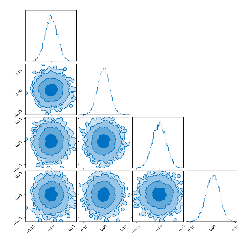
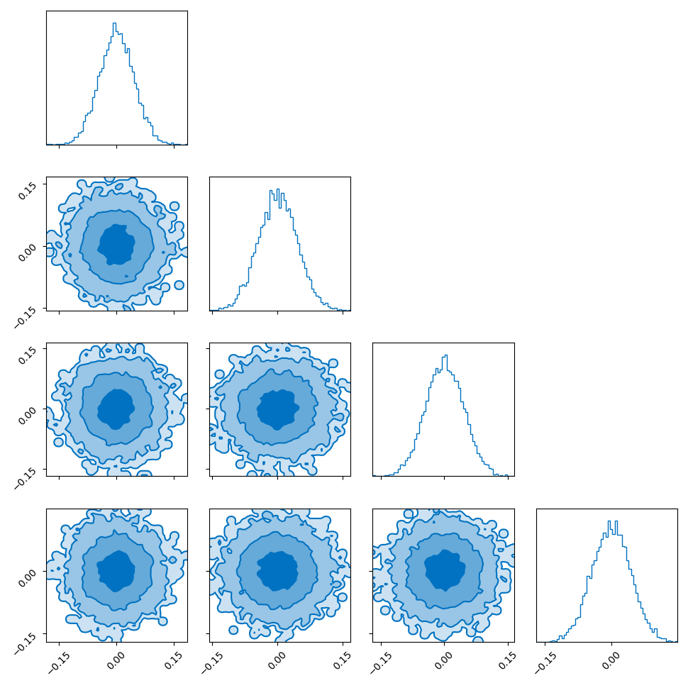
I showed the converse of this in my post on hyperspherical and hyperbolic VAEs, where if you sample uniformly on the unit sphere in high dimensions (~500) the distribution you get out in the marginals (the corner plot) is indistinguishable from those of a similarly dimensional gaussian.
So you get this kind of Faustian bargain where you can either:
- Making the step size/width of the proposal small, so that samples that are close/on the sphere stay close/on the sphere. But then exploring the hall space/distribution will be very inefficient, making the process take exponentially longer.
- Making the step size/width of the proposal large, so you can quickly explore the whole space, but have a low efficiency of having samples fall in the typical set, making the process take exponentially longer….
Walking home drunk is not an efficient way to get home (kinda)
Closely linked to the above issue is how the efficiency of the stochastic process (sometimes referred to as a drunken walk process) scales with dimension. For a \(d\)-dimensional distribution the efficiency of the process assuming an target efficiency of ~0.234 (23.4\%) (refs Optimal scaling of discrete approximations to Langevin diffusions - Roberts, Rosenthal (1998), Investigating the Efficiency of the Metropolis Algorithm - Dou, Li, Wang (2024)) the optimal step size for RWM scales as \(d^{-1/2}\) and efficiency (or number of steps) as \(\mathcal{O}(d)\).
Viewing this process as a diffusion process, where the efficiencies relate to how long it takes to reach an equilibrium distribution or a good enough approximation of one, then leaves the door open for us to wonder if other dynamics/processes could scale significantly better?
On possible algorithm that achieves this are the so-called “Langevin algorithms” that model the process via Langevin dynamics. Roberts & Tweedie (1996) showed that the proposal distributions for Langevin-based algorithms could scale as \(d^{-1/3}\) and the number of steps as \(\mathcal{O}(d^{1/3})\)! Which for high-dimensional sampling is a complete game changer when it comes to efficiency.
A sneak peak at the goal of the post: An intuitive picture of Langevin Monte Carlo
Imagine the sampling trajectories of MCMC as people trying to find their way home after a long night out. They are in their neighborhood, but they are delirious and have no sense of direction.
The RWM drunkards have lost their glasses in the mayhem of the night, and thus have completely failing eyesight. They pick a house at random nearby, stumble to the door, and are then close enough to check the house number on the door (the probability density). If that number is closer to their own address, they feel a sense of “positive feedback” and are likely to stay there for a moment. But then, forgetting everything, they stumble toward another random house. As this process repeats they have an unconcious positive feedback ‘pull’ towards the right house number. They are essentially “diffusing” through the neighborhood. Because they don’t know which way the numbers are increasing or decreasing, they spend a massive amount of time walking in circles or heading toward the wrong end of the street.
The Langevin (LMC) Drunkard is just as tired, but they’ve managed to keep their glasses on. They can actually read the street signs. They notice the house numbers are increasing as they walk East, so they purposefully start walking East (the Drift). They are still drunk, so they still trip over the curb or weave side-to-side randomly (the Diffusion), but their average movement is a direct line toward their front door.
In a 1D street, the RWM drunkard might eventually find home. But imagine a 100-dimensional neighborhood (imagine Los Angeles in Blade Runner 2049 on steroids).
The RWM drunkard is almost certain to take a step that leads them away from their house because there are so many “wrong” directions to choose from.
The LMC drunkard, even with a slight stagger, has a compass (the Gradient). They ignore the 99 wrong directions and focus their energy on the one direction that actually matters.
More formally, LMC introduces a drift into the proposal distribution or gradient flow using the gradient of the target probability density but otherwise uses the same accept-reject as the typical MHMCMC algorithm. And even more formally … is the rest of this post.
Below is a GIF showing how RWM and LMC converge on a target (same step size, set so that RWM is purposefully bad, but even then the LMC is fine).


We will try to explain, motivate and show how we construct the below algorithm and that it in fact has an equilibrium distribution that matches our target.
Metropolis-Adjusted Langevin Algorithm
- Initialise:
- Have a target density you want to sample from \(f(x)\) (known up to a normalising constant),
- Define the potential energy as the negative log-density: \(U(x) = - \log f(x)\),
- Manually choose a starting point \(x_0\),
- Pick a step size \(\epsilon > 0\),
- Pick the number of samples to generate \(N\).
- For each iteration \(n\) / Repeat \(N\) times:
- Langevin proposal steps:
- Compute the gradient of the log-density at the current state: \(\nabla \log f(x_n)\)
- Generate a proposal point \(x^*\) using a drift term plus noise: \(x^* = x_n + \frac{\epsilon}{2} \nabla \log f(x_n) + \sqrt{\epsilon} \eta\) where \(\eta \sim \mathcal{N}(0, I)\)
- Metropolis Hastings correction steps:
- Compute the proposal densities: \(q(x^* \mid x_n) = \mathcal{N}\left(x^* ; x_n + \frac{\epsilon}{2} \nabla \log f(x_n),\epsilon I\right)\) \(q(x_n \mid x^*) = \mathcal{N}\left(x_n ; x^* + \frac{\epsilon}{2} \nabla \log f(x^*),\epsilon I\right)\)
- Compute the acceptance probability: \(\alpha = \min\left(1, \frac{f(x^*) q(x_n \mid x^*)}{f(x_n) q(x^* \mid x_n)}\right)\)
- Draw a random number \(u \sim \text{Uniform}(0, 1)\)
- Accept or reject:
- If \(u \le \alpha\), set \(x_{n+1} = x^*\)
- If \(u > \alpha\), set \(x_{n+1} = x_n\)