Flow matching for multi-modal density estimation and image generation
Published:
In this post, I’ll give an practical introduction to flow matching for the sake of estimating complicated sample distributions and image generation.
Resources
As usual, here are some of the resources I’m using as references for this post. Feel free to explore them directly if you want more information or if my explanations don’t quite click for you.
- Flow Matching Guide and Code - Yaron Lipman, Marton Havasi, Peter Holderrieth, Neta Shaul, Matt Le, Brian Karrer, Ricky T. Q. Chen, David Lopez-Paz, Heli Ben-Hamu, Itai Gat
- MIT 6.S184: Flow Matching and Diffusion Models - Peter Holderrieth
- A Visual Dive into Conditional Flow Matching - Anne Gagneux, Ségolène Martin, Rémi Emonet, Quentin Bertrand, Mathurin Massias
- Flow Matching for Generative Modeling - Yaron Lipman, Ricky T. Q. Chen, Heli Ben-Hamu, Maximilian Nickel, Matt Le
- Neural Ordinary Differential Equations (continuous normalising flows) - Ricky T. Q. Chen, Yulia Rubanova, Jesse Bettencourt, David Duvenaud
Table of Contents
- Motivation
- Core Idea
- Constructing the loss
- Checkerboard density dimensional and modal scaling behaviour
- Generating MNIST-like images with conditional flow matching
- Conclusion
Motivation
In a previous post I explained the use of Variational Autoencoders and how there probabilistic nature allowed us to sample “new” images from the MNIST dataset. However, this came with a few caveats:
- We were not able to easily enforce a specific structure on the learnt latent space. The latent space or the values represented in the bottleneck were learnt as part of the training.
- Similar to the previous point, say we were in a true variational inference context. We may want a specific likelihood and prior for our latent space that was informed from physical parameters. This would not be possible with a variational autoencoder without modifications that wouldn’t make it a standard variational autoencoder anymore.
- The learnt distributions were fixed (gaussian) and failed to capture some details that maybe a more complex distribution would be able to capture. But we couldn’t specify this as it seemed like there was no way to form a good distribution without knowing what it was beforehand.
Many of the capabilities of the above can be handled by a relatively recent (2022) machine learning architecture/density estimation approach called Flow Matching. Initially introduced by Lipman et al.1 as an evolution of continuous normalising flows, it retains much of the expressibility of continuous flows with much more stable training and no need to explicitly solve ODEs.
The training and setup is now so simple, I personally wasted a lot of time trying to understand flow matching “better” because I didn’t think I had the right interpretation. Going into Riemannian space optimal transport for example, just to learn that I had the right idea all along. I am thus only going to introduce the final result here, and not much of the underpinning theory (leaving that for the post on SBI where some extra detail is needed) as I think knowing it will only initially get in the way of developing an intuition.
Core Idea
Flow matching is inherently a simulation-based approach that requires samples from the target distribution. The first step in developing a flow representation of this target is to investigate the conditional paths of the samples. Where all the samples from the base distribution flow into a single sample in the target. Mathematically, if we assume that our base distribution is a normal distribution with mean \(\mu_0\) and covariance \(\Sigma_0\), we can describe the probability of a given point during the transform at time \(t\), \(x_t\), for a given point in the target distribution \(x_1\) as,
\[\begin{align} p_t(x_t | x_1, t) = \mathcal{N}(x_t | \mu_0 + t \cdot (x_1 - \mu_0), (1-t)^2 \cdot \Sigma_0). \end{align}\]Or more simply we can imagine transforming a given point in the base distribution \(x_0\),
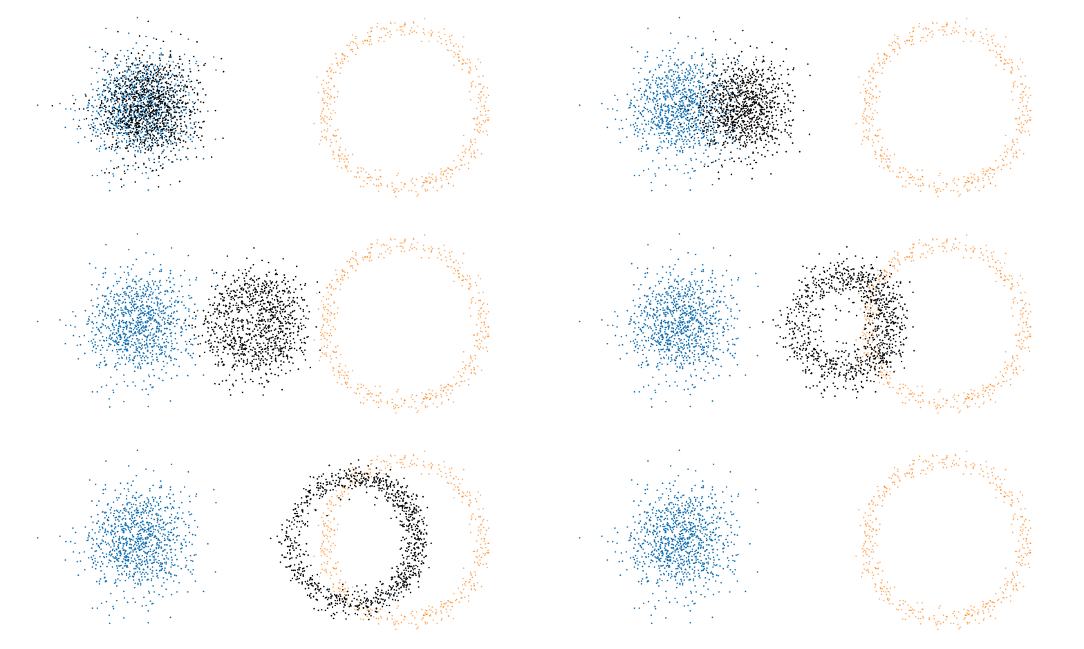
\[\begin{align} x_t = x_0 + t \cdot (x_1 - x_0). \end{align}\]For a visualisation of this you can look at the below GIFs with the given target sample highlighted in red.
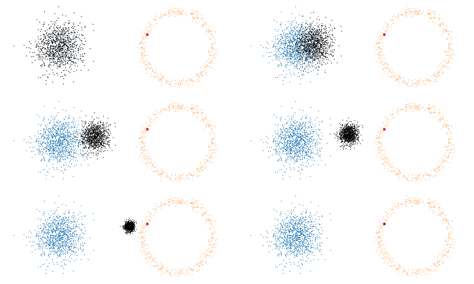
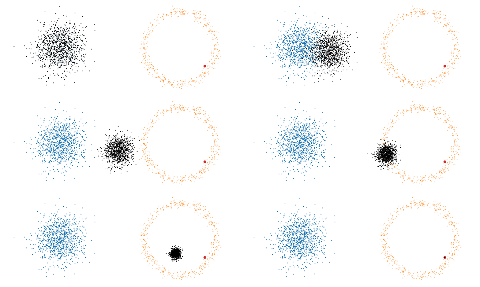
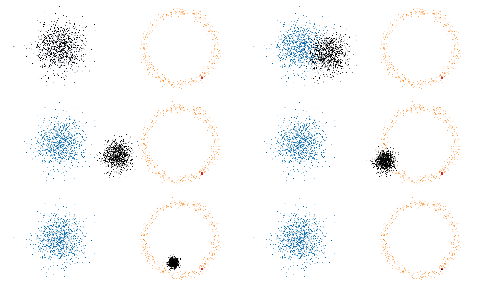
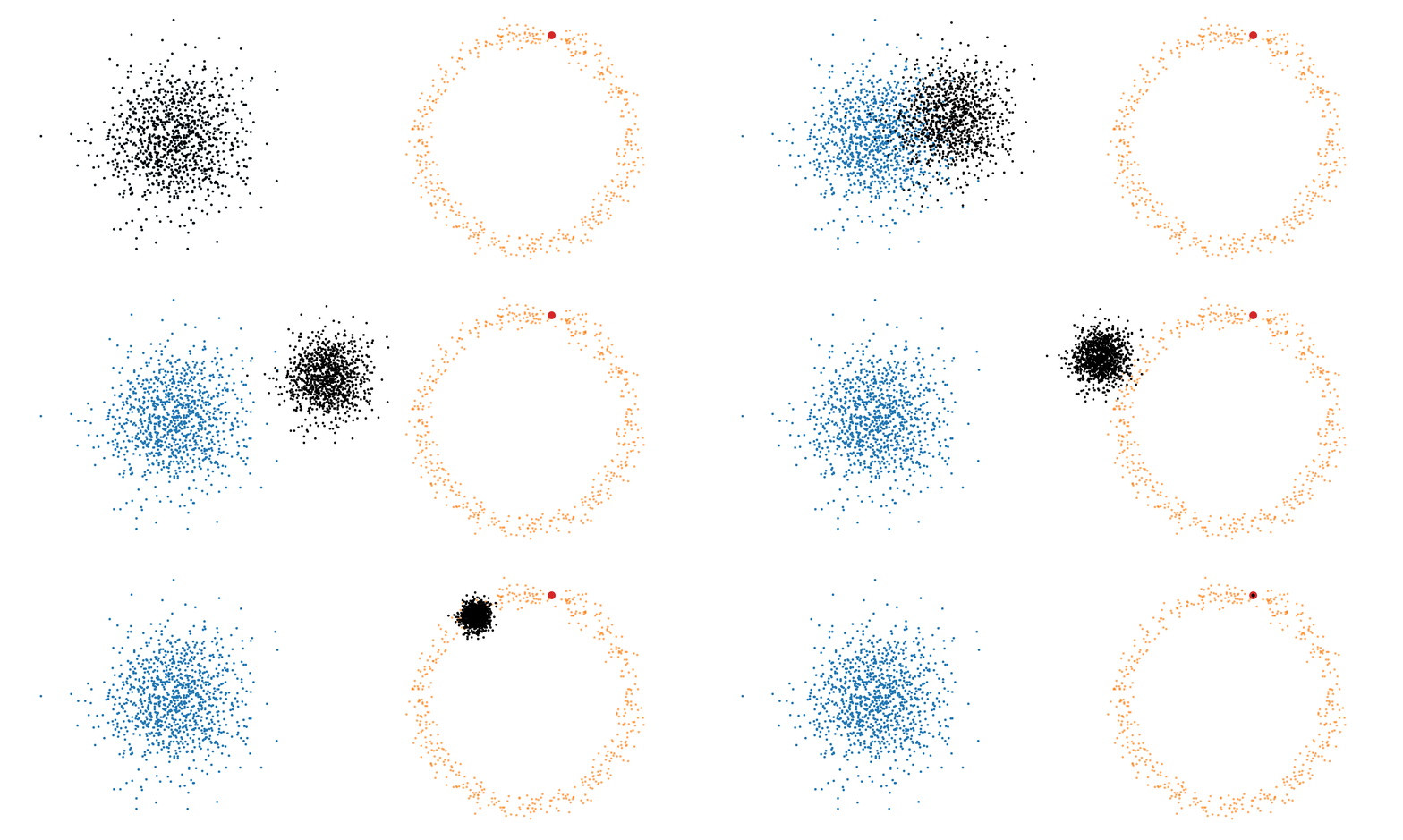
The probability path satisfied the conditions,
\[\begin{align} p_t(x_t | x_1, t) =\begin{cases} \mathcal{N}(x_t | \mu_0, \Sigma_0), & \text{if }t\text{ = 0} \\ \delta(x_t - x_1), & \text{if }t\text{ = 1} \end{cases} \end{align}\]The underlying vector field \(u_t\) that is driving this is then just2,
\[\begin{align} u_t(x_t | x_1, t) = \frac{x_1 - x_t}{1-t} \end{align}\]This just means that all the points are following straight lines more simply given via the transform equation above.
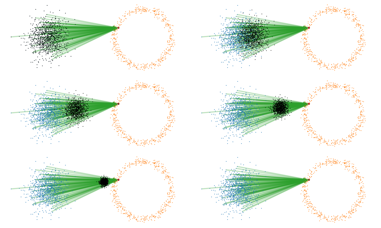
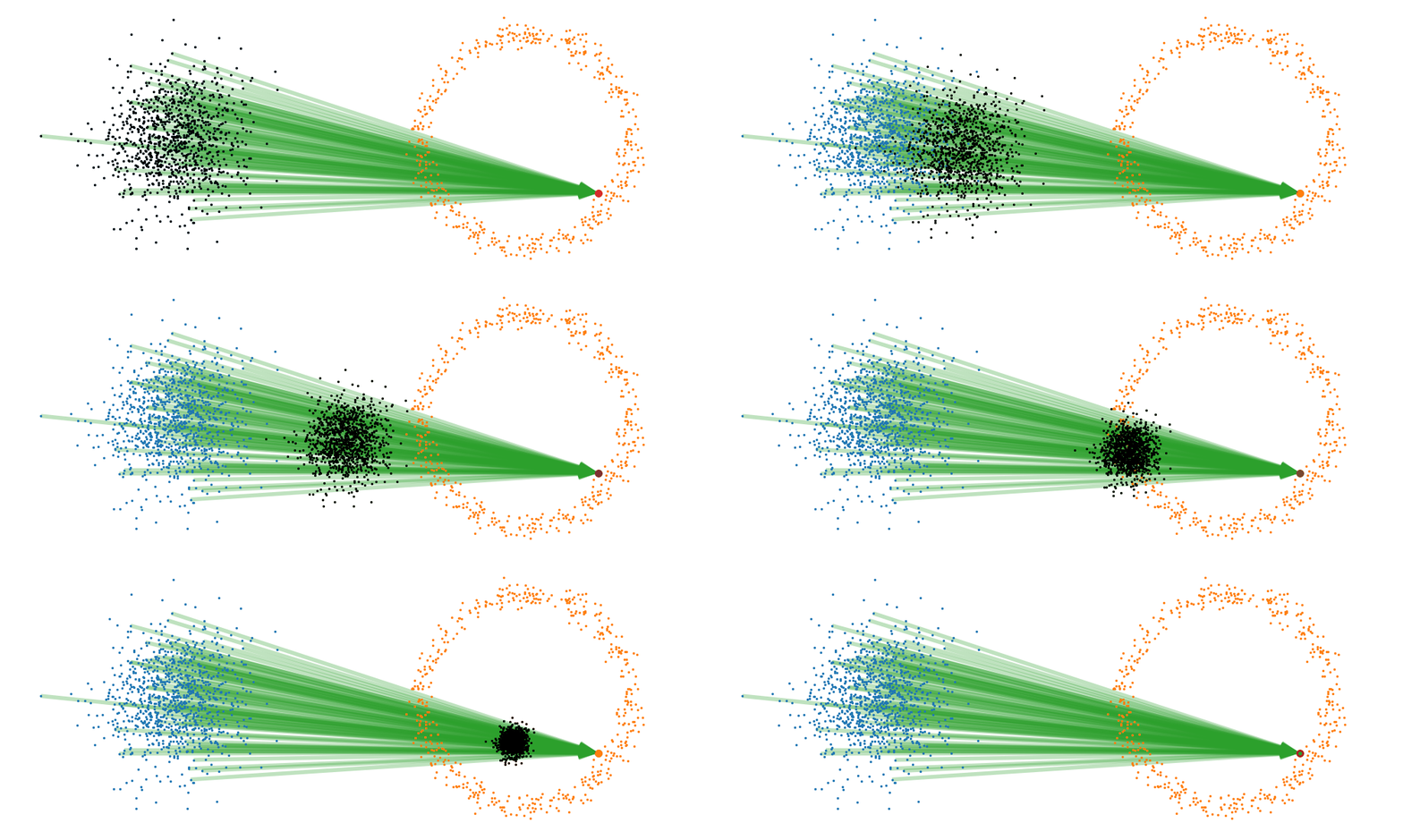
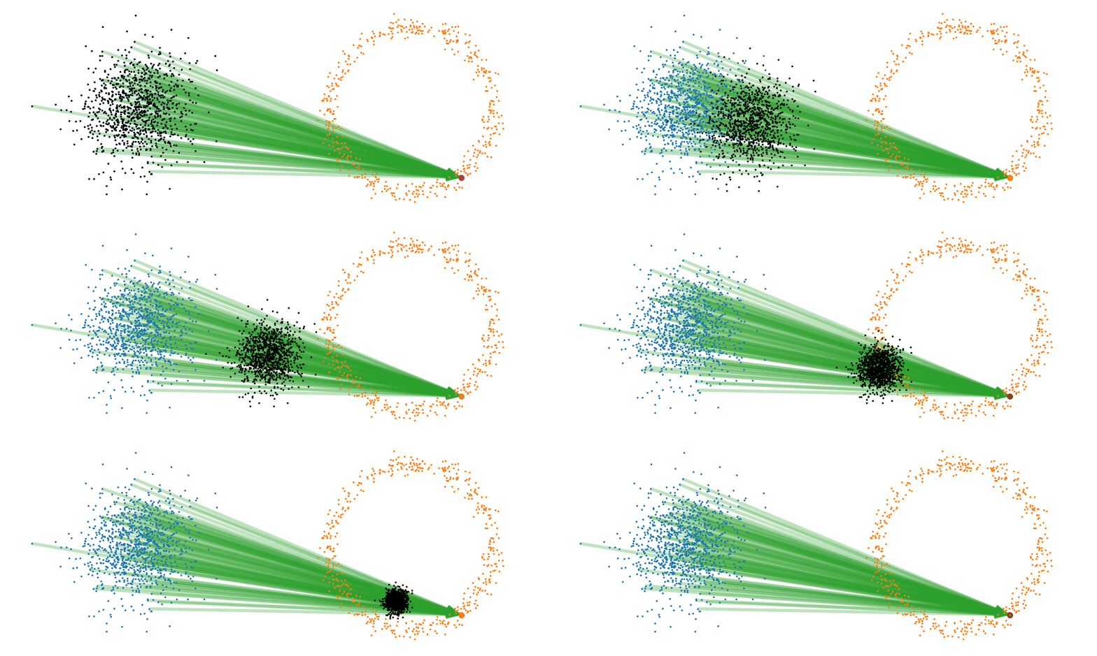
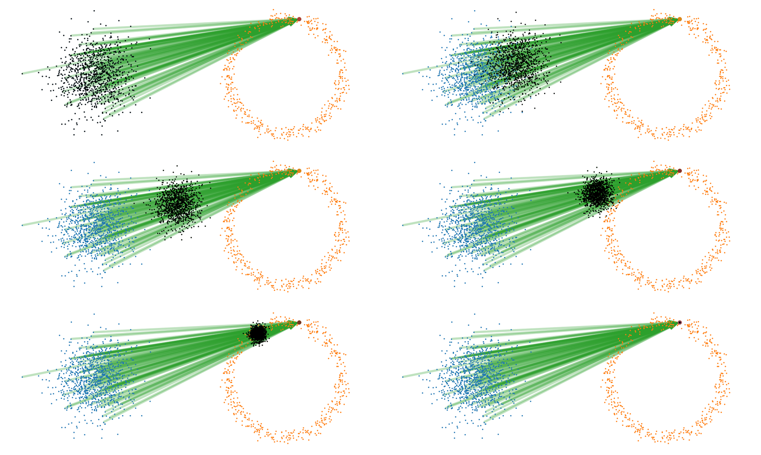
If we directly look at the vector field, not just individual trajectories, you can see that everywhere is just pointing towards the target distribution sample.
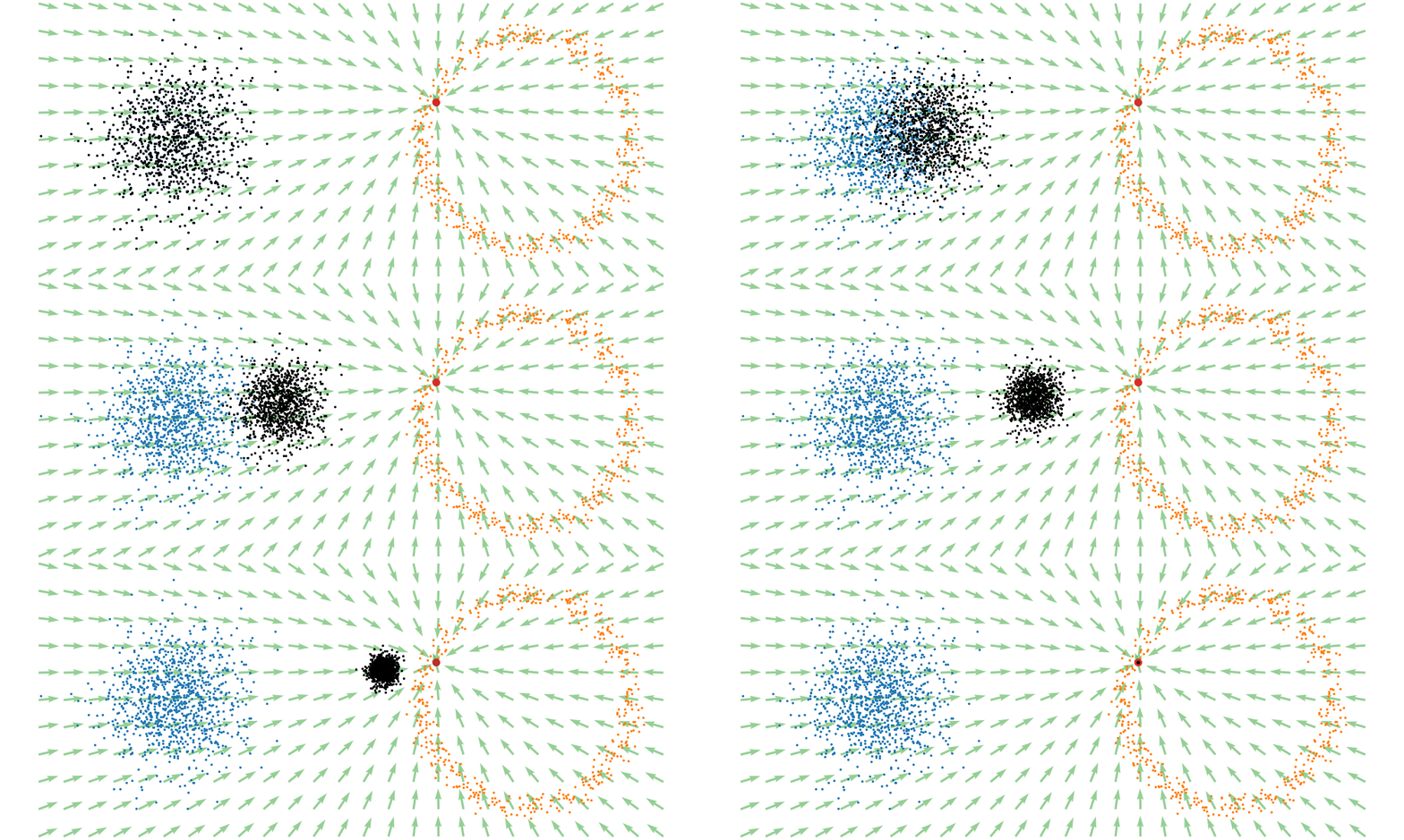
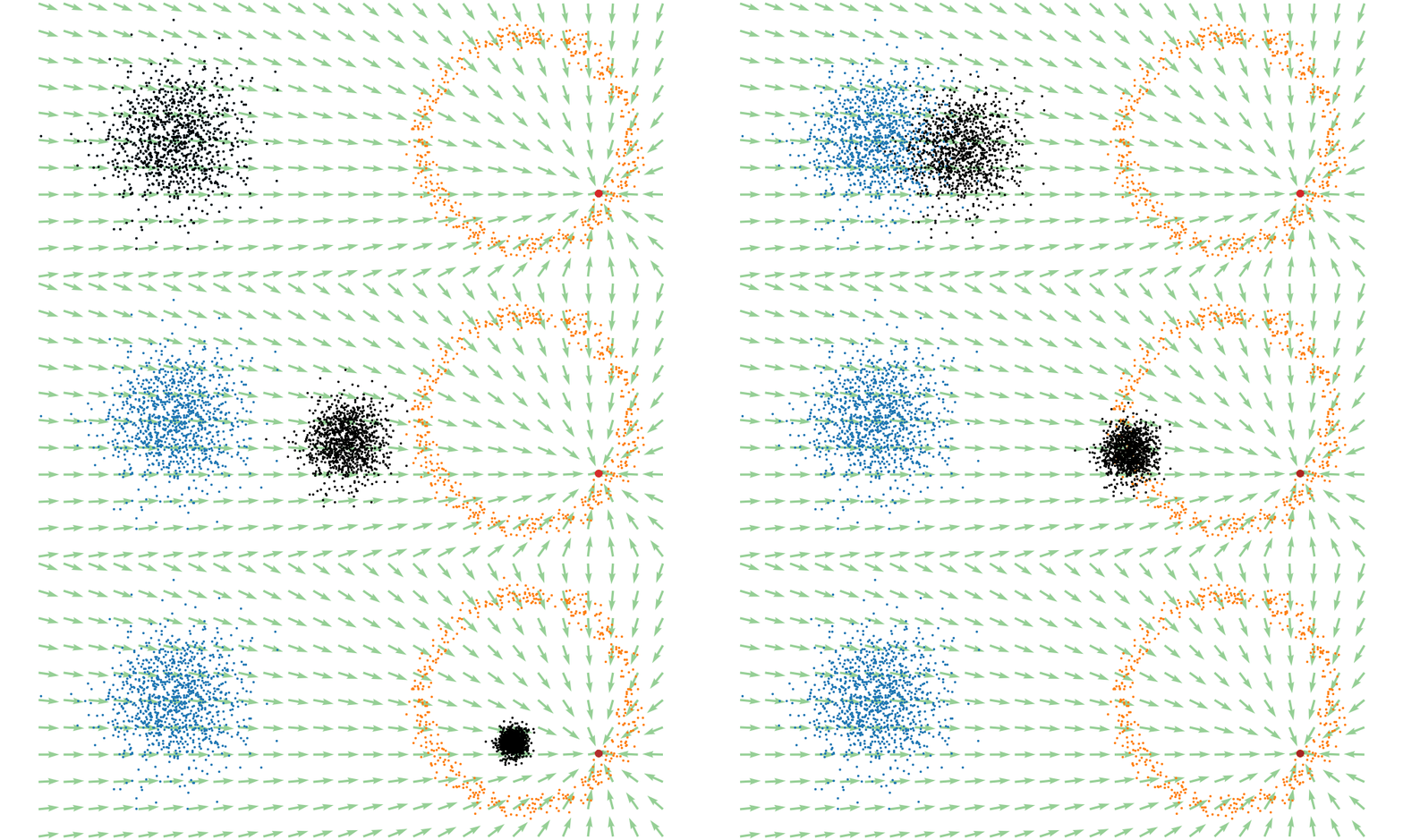
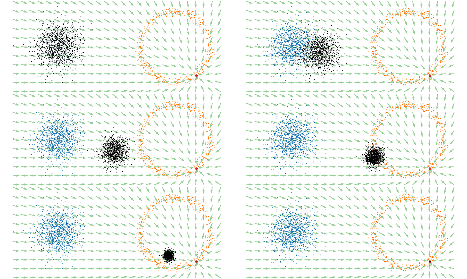
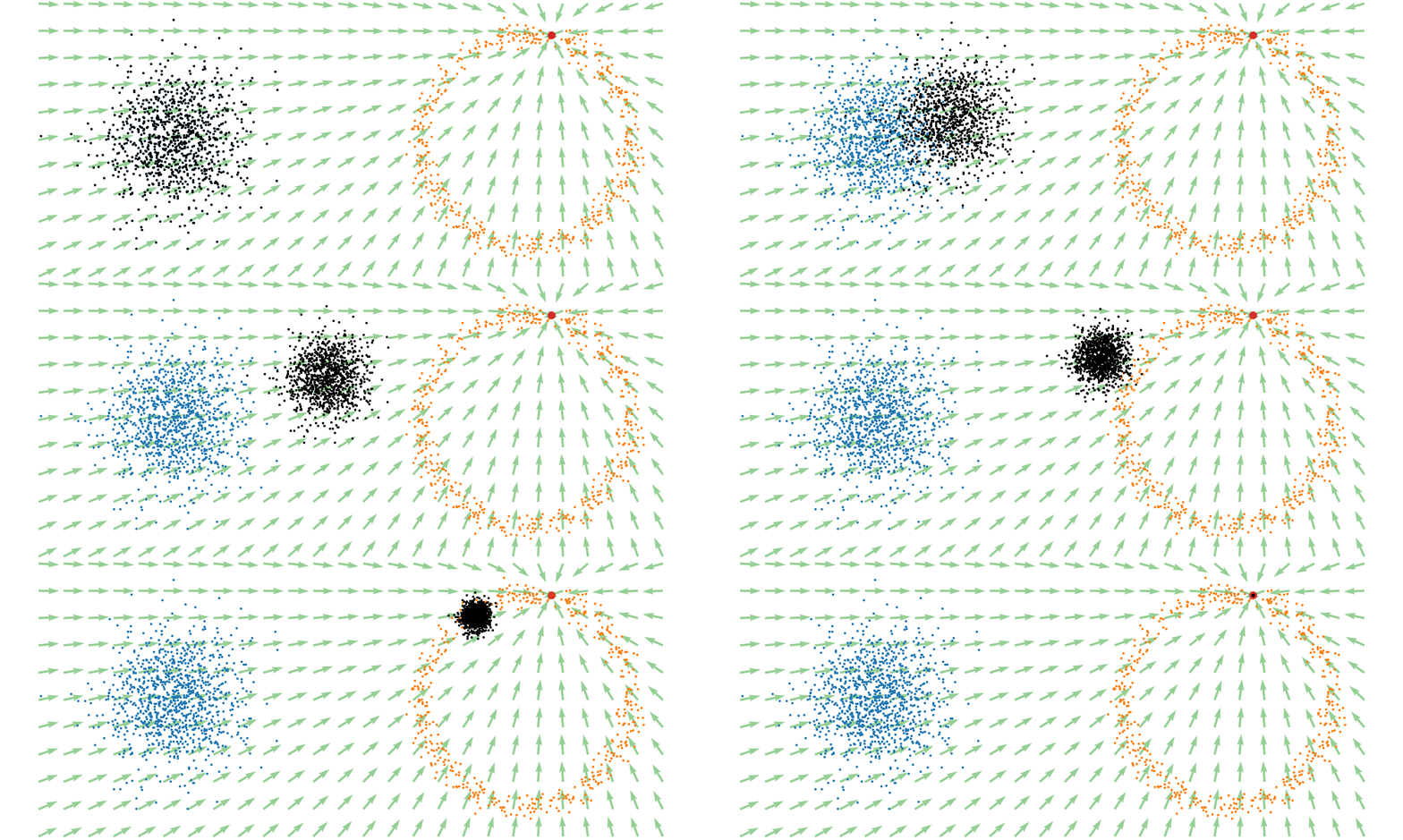
This doesn’t take into account the samples from the base distribution? The vector field we want is of course \(u_t(x_t)\), not conditioned with respect to a specific target sample. We can take out this dependence by marginalising it out with respect to the probability path we defined above,
\[\begin{align} u_t(x_t ; t) &= \int dx_1 u_t(x_t ; t, x_1) p(x_1 | x_t) \\ &= \int dx_1 u_t(x_t ; t, x_1) \frac{p(x_t | x_1)p(x_1)}{p(x_t)} \\ \end{align}\]Which we can estimate with a couple rounds of monte carlo integration,
\[\begin{align} u_t(x_t ; t) &= \int dx_1 u_t(x_t ; t, x_1) \frac{p(x_t | x_1)p(x_1)}{p(x_t)} \\ &\approx \frac{1}{N_i} \sum_s^{N_i} u_t(x_t ; t, x_1) \frac{p(x_t | x_1^i)}{p(x_t)}, \\ \end{align}\]and with the same set of samples from the target distribution,
\[\begin{align} p(x_t) &= \int dx_1 p(x_t | x_1)p(x_1) \\ &\approx \frac{1}{N_i} \sum_i^{N_i} p(x_t | x_1^i). \end{align}\]This gives us the following estimates for the vector field that transforms our base distribution to our target distribution.
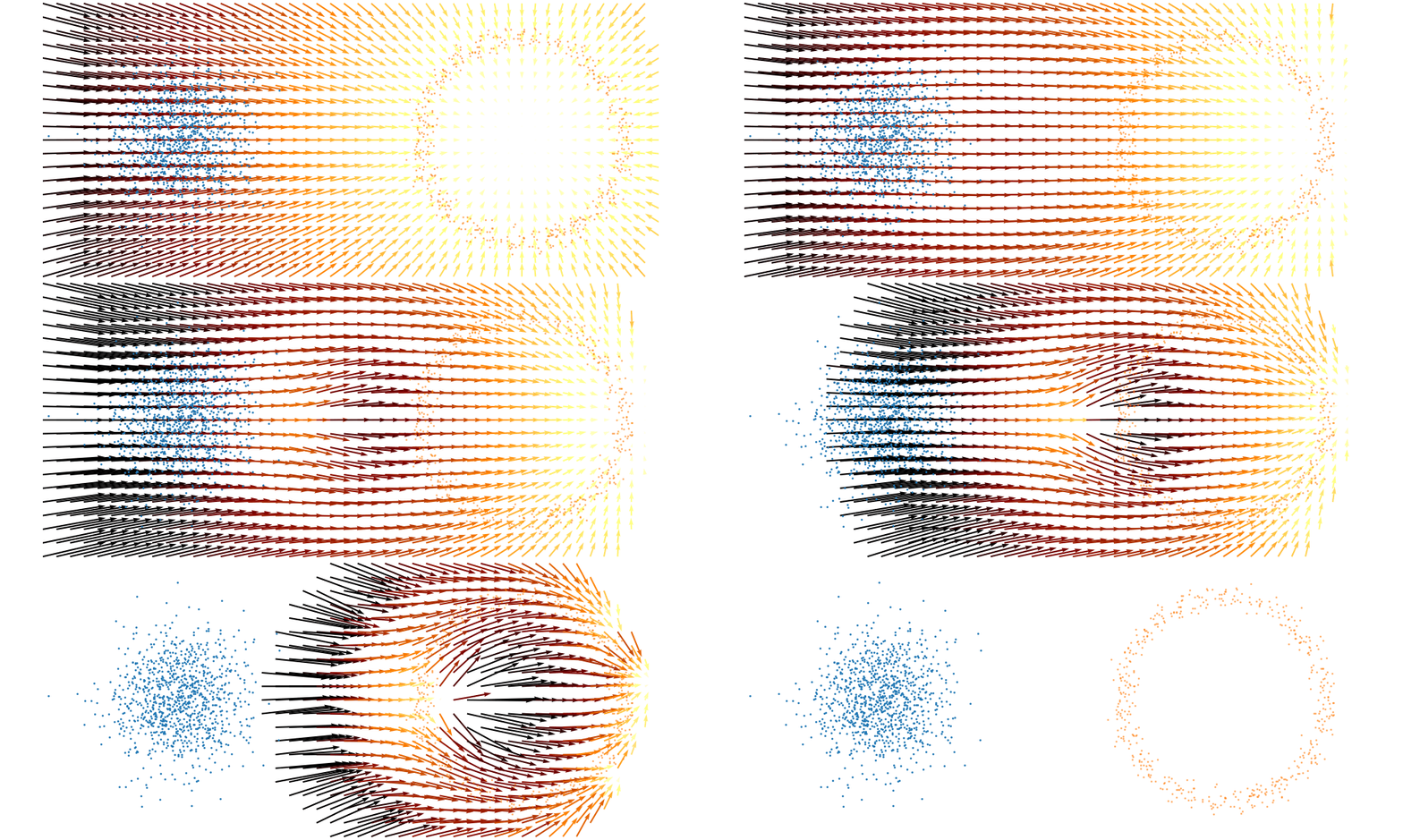
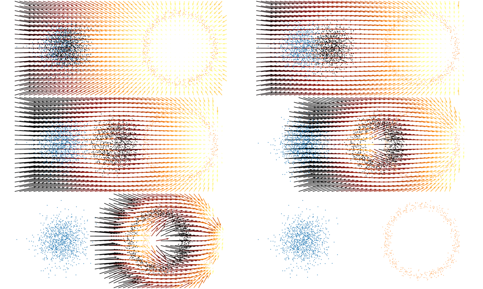
And we can look at how the vector field is directly acting on the points themselves3.
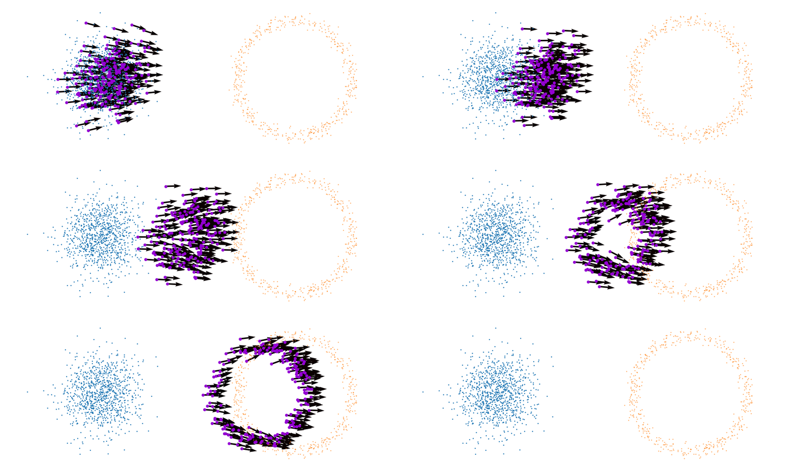
But mathematically the points on the left aren’t even in the same space as the right (the space of \(x_0\) is not the same as \(x_1\) i.e. \(x_0 \neq x_1\)). Although they look that way, because of the way that I’ve put them in the gifs. What we’re actually doing under the hood is transforming the space itself. The closest analogy I can come up with is that for whatever reason, we are interested in how a surfer is riding a wave (the samples), that were originally standing on a surfboard (space being transformed), and the wave (vector field) is pushing the board (space the samples inhabit) not exactly the surfer (samples)4. And the surfer (samples) are in the exact same position relative to the board (base distribution sample space).
So, we can also look at how the samples actually just inhabit the space deforming, not exactly samples moving through a static space. As more correctly shown below.
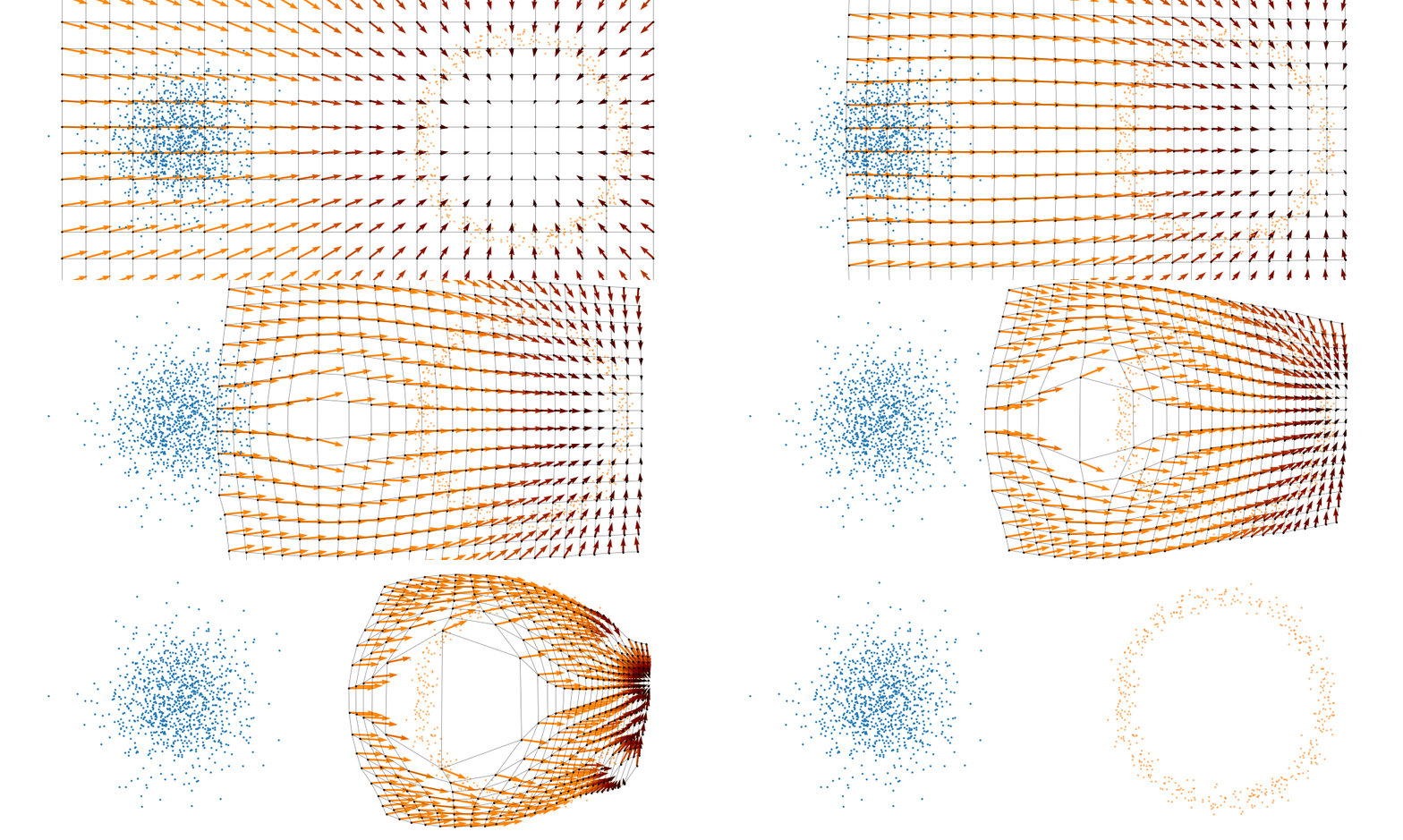
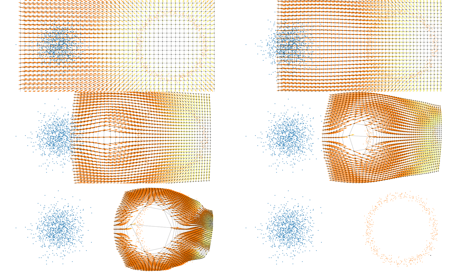
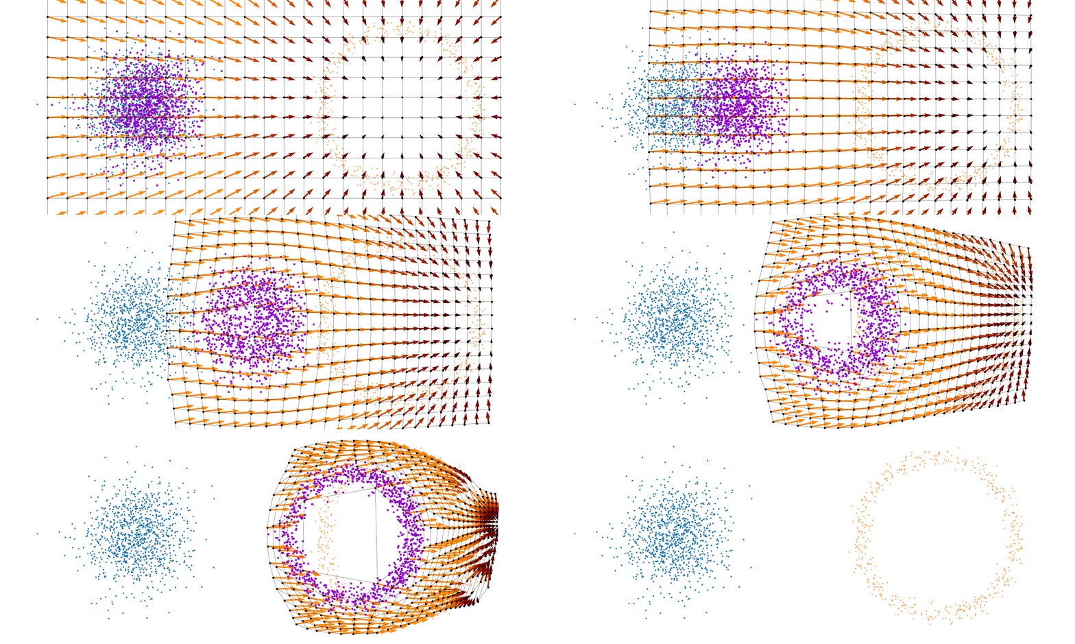
But this approach would not be feasible for large dimensions or really pathologically shaped distributions. So instead, we try to represent the vector field with a neural network. And boom, that’s flow matching.
Here’s one I prepared earlier for the above example.
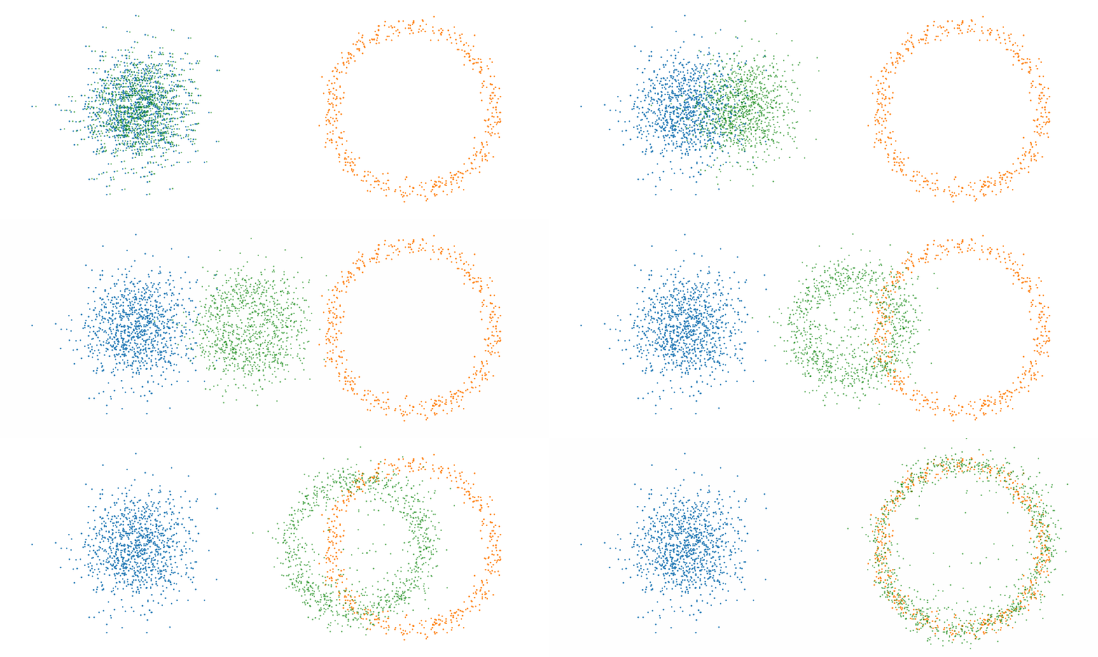
However, if we want to avoid the monte carlo estimation, then how do we tell the network how to improve, i.e. what should we make the loss?
Construction of the conditional flow matching loss
What we would want to do is called the flow matching loss. We sample in time, the base distribution samples and the target distribution samples, and minimise the difference between our approximated vector field \(v_t^\varphi\) and the exact vector field \(u_t\).
\[\begin{align} L_{FM}(\varphi) = \mathbb{E}_{t, X_t}||v(x_t; t, \varphi) - u_t(x_t;t)||^2 \end{align}\]Where the double bars and square denote the 2-norm. But this requires that we have \(u_t\), which kind of defeats the point of making an approximate version…
And now instead of going through the full derivation5 I’m just going to motivate what will essentially be an Ansatz. The following is called the conditional flow matching loss.
\[\begin{align} L_{CFM}(\varphi) = \mathbb{E}_{t, X_t, X_1}\vert\vert v(x_t; t, \varphi) - u_t(x_t|x_1;t)\vert\vert^2 \end{align}\]We can then simplify this by plugging in our version of \(u_t(x_t\vert x_1;t)\),
\[\begin{align} L_{CFM}(\varphi) &= \mathbb{E}_{t, X_t, X_1}||v(x_t; t, \varphi) - u_t(x_t|x_1;t)||^2 \\ &= \mathbb{E}_{t, X_t, X_1}||v(x_t; t, \varphi) - \frac{x_1-x_t}{1-t}||^2 \\ &= \mathbb{E}_{t, X_0, X_1}||v(x_t; t, \varphi) - \frac{x_1-(x_0 + t(x_1-x_0))}{1-t}||^2 \\ &= \mathbb{E}_{t, X_0, X_1}||v(x_t; t, \varphi) - \frac{(1-t)x_1 - (1-t)x_0}{1-t}||^2 \\ &= \mathbb{E}_{t, X_0, X_1}||v(x_t; t, \varphi) - (x_1 - x_0)||^2. \end{align}\]For the above this comes from the fact that if we have a given \(x_0\) and a given \(x_1\) then the vector field between them should literally just be the vector from one to the other \(u = x_1 - x_0\). We’ll stick to the original for ease-of-derivations.
It turns out the gradient of \(L_{FM}\) and \(L_{CFM}\) with respect to \(\varphi\) are the same. Which if so, means that they are effectively the same thing, at least to us. During training we use the gradients, not strictly the value of the loss.
We can show that the two gradients are the same by a little algebraic magic with the conditional flow matching loss.
First I’ll just again note that the average of the vector field with respect to \(p_t(x_t\vert x_1)\) would theoretically give us the exact transformation vector field.
\[\begin{align} u_t(x_t;t) = \mathbb{E}_{X_1}\left[u_t(x|x_1;t) \right] \end{align}\]We can expand the squared norm using some the inner product identity.
\[\begin{align} || A -B ||^2 &= || A -C + C- B ||^2 \\ &= \langle (A - C) + (C - B), (A - C) + (C - B) \rangle \\ &= || A - C ||^2 + 2 \langle A - C, C - B\rangle + || C - B ||^2 \\ \end{align}\]And a little thing with expectations over inner products where \(C\) is not a function of \(A\).
\[\begin{align} \mathbb{E}_{A} \langle C, f(A) \rangle &= \mathbb{E}_{A} \sum_i C_i \cdot (f(A))_i \\ &= \sum_i C_i \cdot \mathbb{E}_{A}(f(A))_i \\ &= \langle C, \mathbb{E}_{A}(f(A))\rangle \\ \end{align}\]Using these, we can expand the conditional flow matching loss.
\[\begin{align} L_{CFM}(\varphi) = \mathbb{E}&_{t, X_t, X_1}||v(x_t; t, \varphi) - u_t(x_t|x_1;t)||^2 \\ = \mathbb{E}&_{t, X_t, X_1}||v(x_t; t, \varphi) -u_t(x_t;t) + u_t(x_t;t)- u_t(x|x_1;t)||^2 \\ = \mathbb{E}&_{t, X_t, X_1} \left[ v(x_t; t, \varphi) -u_t(x_t;t)||^2 \right. \\ &\left. + 2 \langle v(x_t; t, \varphi) -u_t(x_t;t), u_t(x_t;t)- u_t(x|x_1;t)\rangle \right. \\ &\left. + ||u_t(x_t;t)- u_t(x_t|x_1;t)^2 \right] \\ = \mathbb{E}&_{t, X_t, X_1}\left[||v(x_t; t, \varphi) -u_t(x_t;t)||^2\right] \\ &\;\; + 2\mathbb{E}_{t, X_t, X_1}\left[\langle v(x_t; t, \varphi) -u_t(x_t;t), u_t(x_t;t)- u_t(x_t|x_1;t)\rangle\right] \\ &\;\; + \mathbb{E}_{t, X_t, X_1}\left[||u_t(x_t;t)- u_t(x_t|x_1;t)||^2\right] \\ = L&_{FM}(\varphi)\\ &\;\; + 2\mathbb{E}_{t, X_t}\left[\langle v(x_t; t, \varphi) -u_t(x_t;t), u_t(x_t;t)- \mathbb{E}_{X_1|X_t}u_t(x_t|x_1;t)\rangle\right] \\ &\;\; + \mathbb{E}_{t, X_t, X_1}\left[||u_t(x_t;t)- u_t(x_t|x_1;t)||^2\right] \\ = L&_{FM}(\varphi)+ \mathbb{E}_{t, X_t, X_1}\left[||u_t(x_t;t)- u_t(x_t|x_1;t)||^2\right] \\ \end{align}\]And the second term here doesn’t depend on \(\varphi\) so \(\nabla_\varphi L_{CFM}(\varphi) =\nabla_\varphi L_{FM}(\varphi)\).
Checkerboard density: Dimensionality and modal scaling behaviour
Now let’s look at a full example. Let’s say that for whatever reason we want to create a flow representation of the following sample distribution.
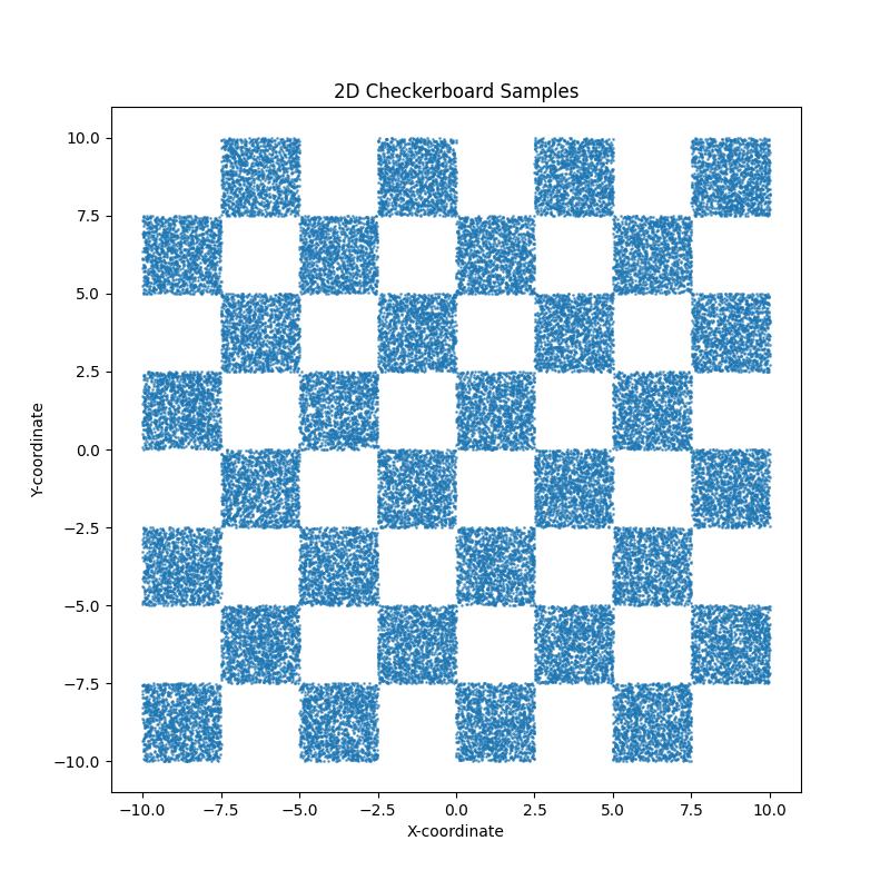
With typical approaches, they would not have great time. As the distribution is extremely multi-modal. But to a flow matching model, this is pretty simple. The actual object that we are modelling is the vector field transporting the samples, which is just a function that we need to approximate with inputs and outputs. So, we can throw a pretty standard MLP network in as our approximate vector field.
from torch import nn
import torch

class Block(nn.Module):
    def __init__(self, channels=512):
        super().__init__()
        self.ff = nn.Linear(channels, channels)
        self.act = nn.ReLU()

    def forward(self, x):
        return self.act(self.ff(x))

class FlowMLP(nn.Module):
    def __init__(self, channels_data=2, layers=5, channels=512):
        super().__init__()

        self.in_projection = nn.Linear(channels_data, channels)

        concat_dim = channels + channels
        self.concat_projection = nn.Linear(concat_dim, channels)

        self.blocks = nn.Sequential(*[
            CondBlock(channels) for _ in range(layers)
        ])
        self.out_projection = nn.Linear(channels, channels_data)

        self.t_mlp = nn.Sequential(
            nn.Linear(1, 128),
            nn.ReLU(),
            nn.Linear(128, channels)
        )


    def forward(self, x, t):

        x = self.in_projection(x)
        t = t.unsqueeze(-1)
        t = self.t_mlp(t) # Learn an embedded depency on t

        # Concatenate and project
        h = torch.cat([x, t], dim=-1)
        h = self.concat_projection(h)

        # Pass through MLP
        h = self.blocks(h)
        h = self.out_projection(h)
        return h
Our training loop is then just implementing the loss that we have above for checkerboard_samples.
from tqdm.notebook import tqdm, trange

training_steps = 2_000

optim = torch.optim.AdamW(model.parameters(), lr=1e-3)
batch_size = 256
pbar = trange(training_steps)
losses = []
for i in pbar:
    # Selecting random batches of our target distribution to lower
        # the computational cost
    x1 = checkerboard_samples[torch.randint(data.size(0), (batch_size,))]

    # Sampling the same number samples from the base distribution
    x0 = torch.randn_like(x1)

    # Calculating x_1 - x_0
    target = x1 - x0

    # Sampling time
    t = torch.rand(x1.size(0))

    # Sample paths / generating X_t
    xt = (1 - t[:, None]) * x0 + t[:, None] * x1

    # Getting out v(x_t;t)
    pred = model(xt, t)  # also add t here

    # Implementing our loss
    loss = ((target - pred)**2).mean()
    loss.backward()
    optim.step()
    optim.zero_grad()
    if (i +1)% 100==0:
        pbar.set_postfix(loss=loss.item())
    losses.append(loss.item())
After training for a few thousand steps I get the following (plus a bonus).
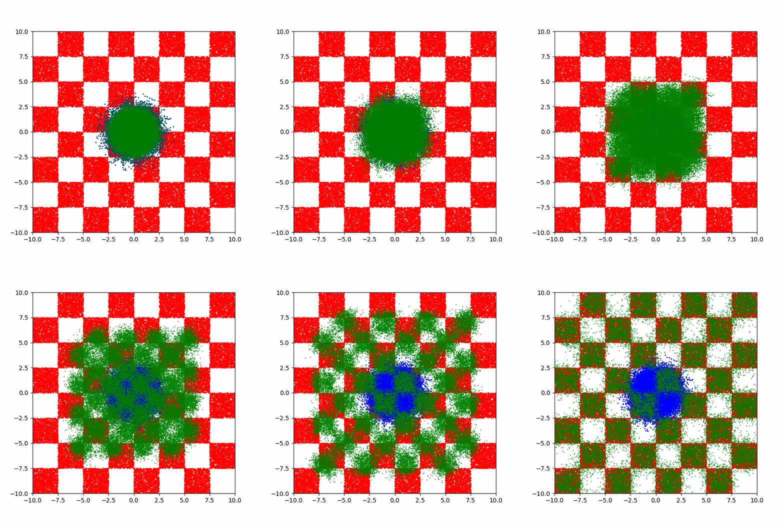
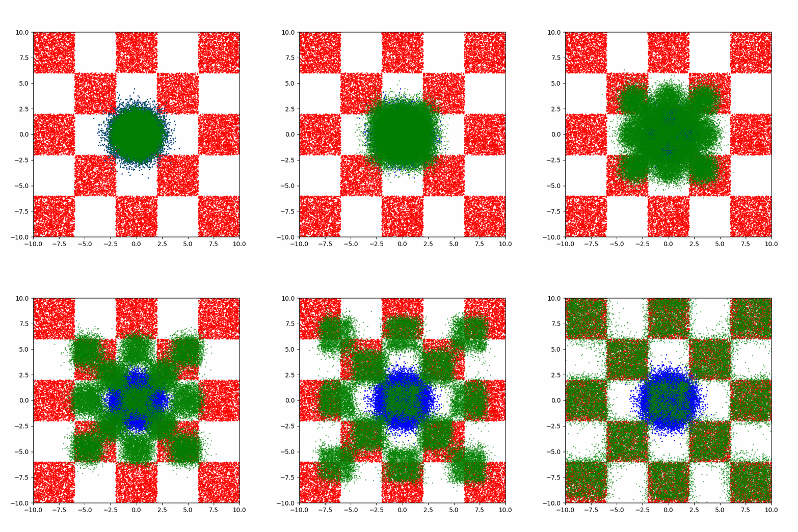
Now it’s not perfect, but that’s just because I couldn’t be bothered training for any longer. But it does allow us to now investigate how the training costs of this kind of approach scales for different aspects of this distribution.
Due to the strict nature of the distribution, we can create a very clear training target of the fraction of samples inside the relevant squares. For my sanity, we’ll say that we want the same level of quality as in the above GIFs. Meaning that the minimum fraction of samples contained with a given square compared to the fraction it should have was XX.
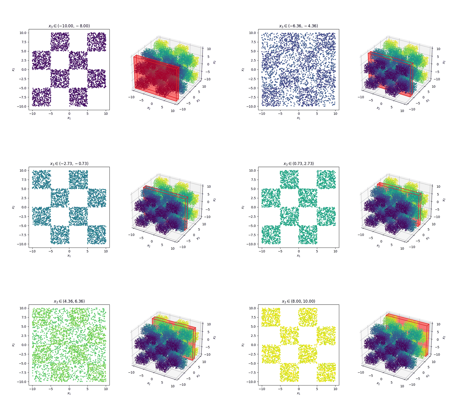
For reference, this is how the samples look in 3D.
** Insert really cool figure showing how many more training steps it takes to go from 8 –> 72 modes **
** Insert really cool figure showing how many more training steps it takes to go from 2 –> 8 dimensions **
** Insert really cool figures showing how many more training steps it takes to go from 2 –> 8 dimensions as a function of the modes **
Generating MNIST-like images (conditional flow matching)
One of the main uses for Flow Matching is image generation. You train the flow on samples of pixel data, where each pixel is it’s own dimension. If we want to train the flow to generate images of 3s then we simply need to give it images of 3s.
from torchvision.datasets import MNIST
import torchvision.transforms as transforms
from torch.utils.data import DataLoader
from torch.utils.data import Subset

mps = False #torch.mps.is_available()

DEVICE = torch.device("mps" if mps else "cpu")
torch.set_default_device(DEVICE)
dataset_path = '~/datasets'
batch_size = 32

mnist_transform = transforms.Compose([
        transforms.ToTensor(),
])

kwargs = {'num_workers': 1, 'pin_memory': True}
# Load datasets
train_dataset = MNIST(dataset_path, transform=mnist_transform, train=True, download=True)
test_dataset  = MNIST(dataset_path, transform=mnist_transform, train=False, download=True)

# Get indices of only "3"s
train_indices = [i for i, t in enumerate(train_dataset.targets) if t == 3]
test_indices  = [i for i, t in enumerate(test_dataset.targets) if t == 3]

# Create filtered datasets
train_dataset_3 = Subset(train_dataset, train_indices)
test_dataset_3  = Subset(test_dataset, test_indices)

# DataLoaders
train_loader_3 = DataLoader(train_dataset_3, batch_size=batch_size, shuffle=True, drop_last=True)
test_loader_3  = DataLoader(test_dataset_3, batch_size=batch_size, shuffle=False, drop_last=True)
and then train in much the same way as we did before. Flattening out the image so we get 784-dimensional ‘samples’.
from tqdm.notebook import tqdm, trange


x_dim  = 784

model = FlowMLP(
    channels_data=x_dim,
    layers=8,
    channels=128)


optimizer = torch.optim.AdamW(model.parameters(), lr=1e-3)

epochs = 1000

tbar = trange(epochs)
losses = []
for epoch in tbar:
    overall_loss = 0
    for batch_idx, (x, _) in enumerate(train_loader_3):

        x1 = x.view(batch_size, x_dim)
        x1 = x1.to(DEVICE)

        x0 = torch.randn_like(x1)

        t = torch.rand(x1.size(0))

        target = (x1 - x0)

        xt = (1 - t[:, None]) * x0 + t[:, None] * x1

        pred = model(xt, t)  # also add t here

        loss = ((target - pred)**2).mean()

        overall_loss += loss.item()

        loss.backward()
        optimizer.step()
        optimizer.zero_grad()

    losses.append(overall_loss/ (batch_idx*batch_size))
    tbar.set_postfix({"Epoch Loss": overall_loss / (batch_idx*batch_size)})
This allows us to generate just images of threes.
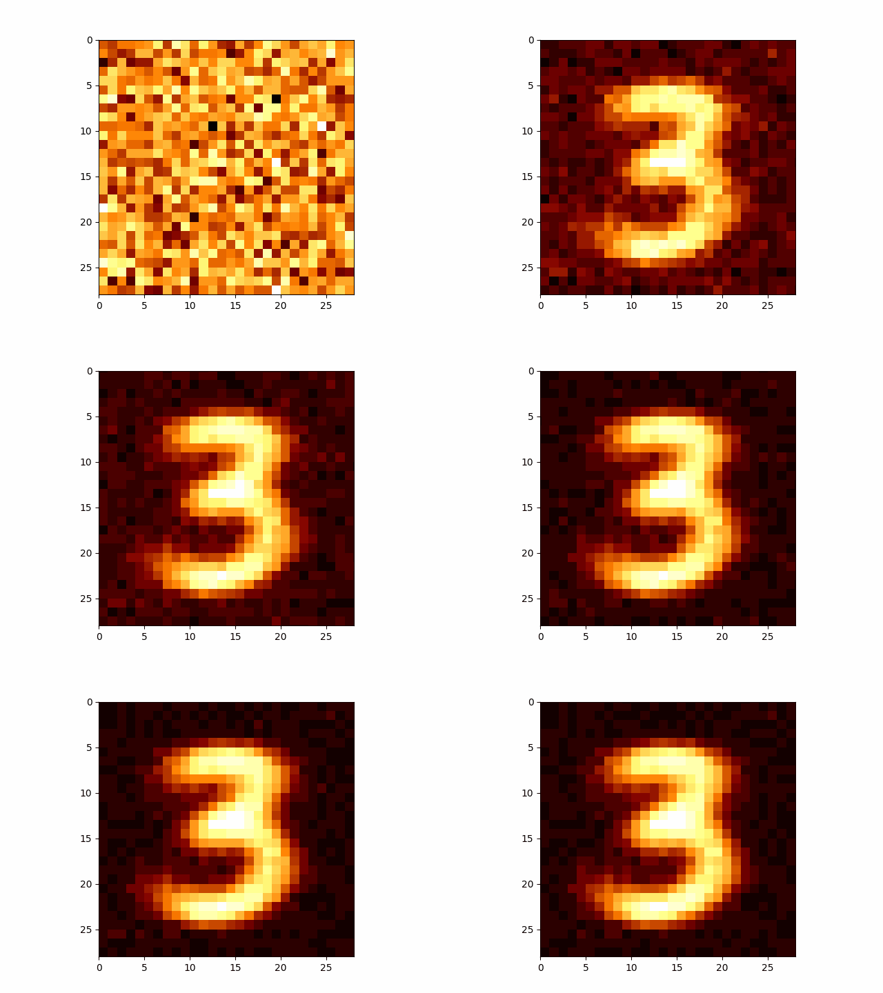
This is a little restrictive though. What if we want to generate images of 4s? Well we’d have to re-run the above for every single number which is a little annoying. And this is just when we have 10 discrete variables.
What if we want to make it more general? Well in that case we would have use conditional flow matching, where we add conditional variables into our representation.
Much like conditional normalising flows (my post on the subject can be found here) our above framework barely changes as the primary goal was to create a representation for the models in our target probability distribution. The labels of whether the numbers are 3s, 4s or etc are not these variables, and simply encode a dependency.
Essentially, if the input is a 3, then we need to change the path that the samples take. i.e. we just need the vector field to have information about the label and that’s it.
Hence, our flow matching network barely changes, we just add an extra embedding for the labels (using the variable y in the below code).
class CondFlowMLP(nn.Module):
    def __init__(self, channels_data=2, layers=5, channels=512, num_classes=10, channels_y=512):
        super().__init__()
        # Projection layers
        self.in_projection = nn.Linear(channels_data, channels)

        self.label_emb = nn.Embedding(num_classes, channels_y)

        # Concatenation projection (data + t + y → hidden)
        concat_dim = channels + channels + channels_y
        self.concat_projection = nn.Linear(concat_dim, channels)

        # Backbone MLP
        self.blocks = nn.Sequential(*[
            Block(channels) for _ in range(layers)
        ])
        self.out_projection = nn.Linear(channels, channels_data)

        self.t_mlp = nn.Sequential(
            nn.Linear(1, 128),
            nn.ReLU(),
            nn.Linear(128, channels)
        )


    def forward(self, x, t, y):
        # Encode inputs
        x = self.in_projection(x)
        t = t.unsqueeze(-1)  # [batch, 1]
        t = self.t_mlp(t) # Learn an embedded depency on t
        y = self.label_emb(y)

        # Concatenate and project
        h = torch.cat([x, t, y], dim=-1)
        h = self.concat_projection(h)

        # Pass through MLP
        h = self.blocks(h)
        h = self.out_projection(h)
        return h
And the training just needs to feed the labels into the model. (If you want to do this yourself this took about 12 minutes on my machine.)
from torchvision.datasets import MNIST
import torchvision.transforms as transforms
from torch.utils.data import DataLoader
from torch.utils.data import Subset

mps = False #torch.mps.is_available()

DEVICE = torch.device("mps" if mps else "cpu")
torch.set_default_device(DEVICE)
dataset_path = '~/datasets'
batch_size = 128

mnist_transform = transforms.Compose([
        transforms.ToTensor(),
])

kwargs = {'num_workers': 1, 'pin_memory': True}
# Load datasets
train_dataset = MNIST(dataset_path, transform=mnist_transform, train=True, download=True)
test_dataset  = MNIST(dataset_path, transform=mnist_transform, train=False, download=True)

# DataLoaders
train_loader_general = DataLoader(train_dataset, batch_size=batch_size, shuffle=True, drop_last=True)
test_loader_general  = DataLoader(test_dataset, batch_size=batch_size, shuffle=False, drop_last=True)

from tqdm.notebook import tqdm, trange


x_dim  = 784

model = CondFlowMLP(
    channels_data=x_dim,
    layers=8,
    channels=128)


optimizer = torch.optim.AdamW(model.parameters(), lr=5e-4)

epochs = 200

tbar = trange(epochs)
losses = []
for epoch in tbar:
    overall_loss = 0
    for batch_idx, (x, label) in enumerate(train_loader_general):

        x1 = x.view(batch_size, x_dim)
        x1 = x1.to(DEVICE)

        x0 = torch.randn_like(x1)

        t = torch.rand(x1.size(0))

        target = (x1 - x0)

        xt = (1 - t[:, None]) * x0 + t[:, None] * x1

        pred = model(xt, t, label)  # also add t here

        loss = ((target - pred)**2).mean()

        overall_loss += loss.item()

        loss.backward()
        optimizer.step()
        optimizer.zero_grad()

    losses.append(overall_loss/ (batch_idx*batch_size))
    tbar.set_postfix({"Epoch Loss": overall_loss / (batch_idx*batch_size)})
Now we can make arbitrary GIFs for whatever numbers we want. The below use the same network, I just feed in the relevant number.
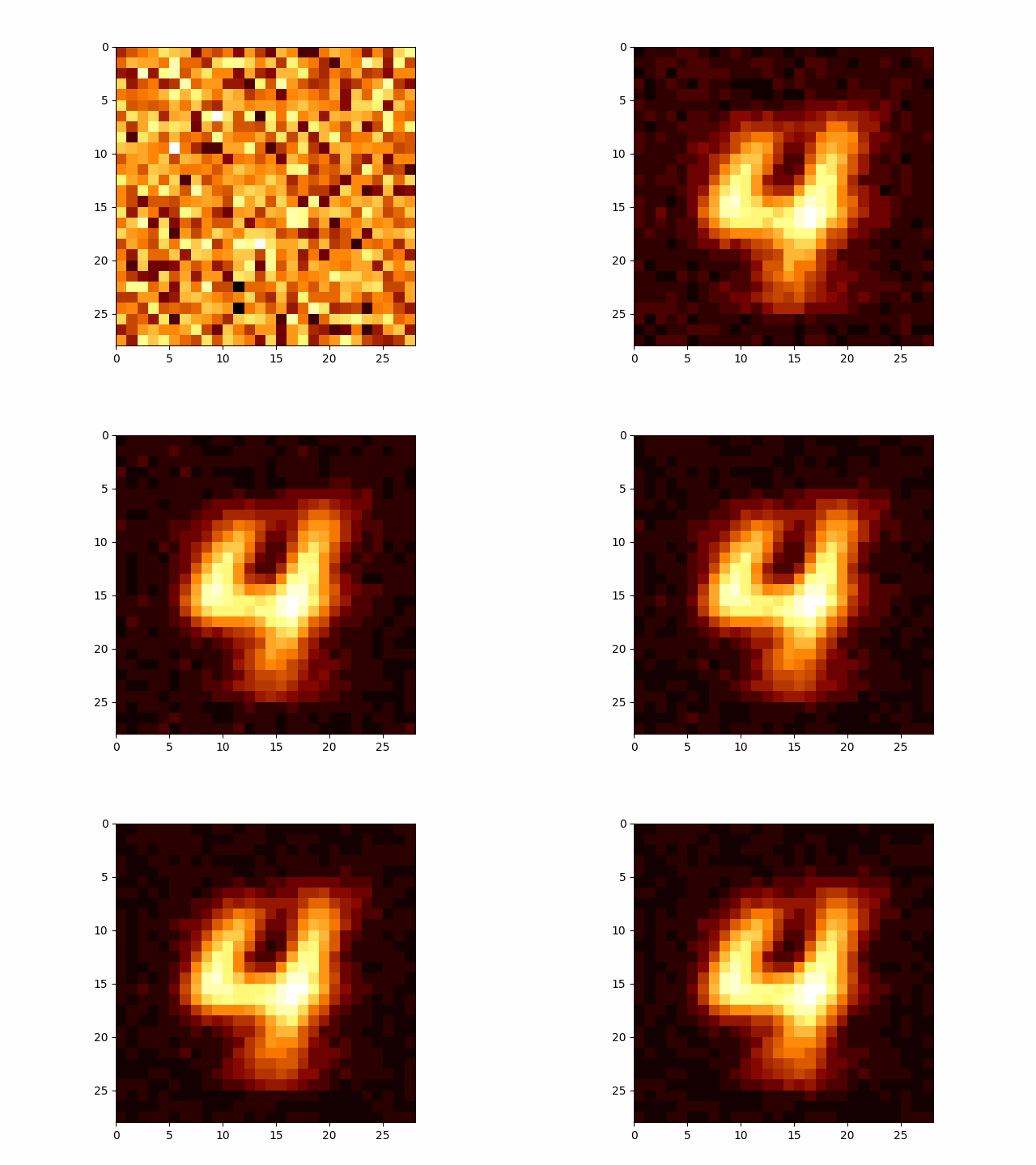
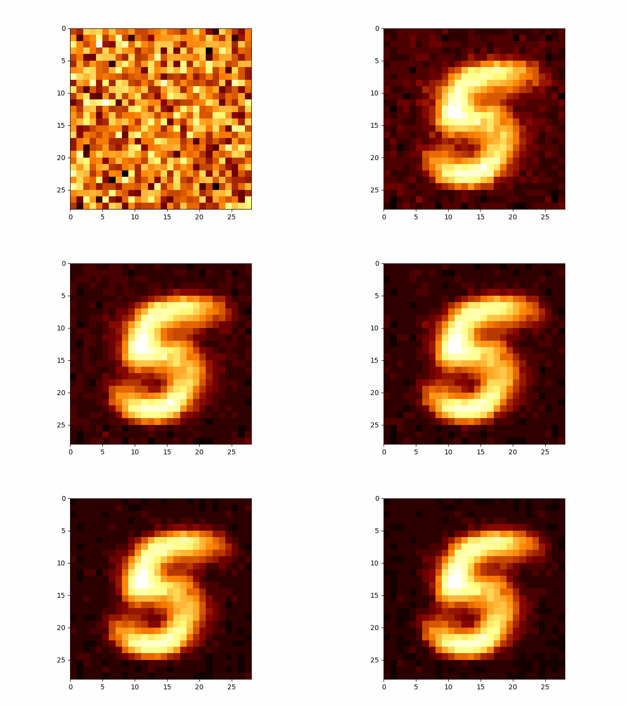
I have to take quite a large average of my values to get these images, which may or may not be related to the reason that DDPM models add extra noise during their training so that they don’t condense onto only a small portion of the overall distribution. But I’m going to leave that for an eventual post on DDPM. If you’re wondering what I’m talking about head on over to Welch Labs video on the topic.
Conclusion
Hope you learnt a little about flow matching! One thing that I left out is that you can get functional representations for the target distribution with this approach, it just requires a little extra work. I’ll go through that in a dedicated post on the SBI method “Flow Matching for Posterior Estimation” otherwise known as FMPE.
And recently there was a fantastic paper released by Meta (Facebook) that goes into much more detail than I will here while also starting from a lower bar of entry. HIGHLY HIGHLY HIGHLY recommend giving it a look https://arxiv.org/abs/2412.06264. ↩
You can rearrange this to just get \(x_1 - x_0\) by plugging in the path above the equation. ↩
I’ve shown this GIF to multiple people and they all say it’s “cute”. I agree. But like why?? ↩
You can tell that I’m a surfer dude…(sarcasm) ↩
Again, I recommend Meta’s paper on the topic https://arxiv.org/abs/2412.06264 if you want something more in-depth. ↩
