In this post, I’ll give an practical introduction to flow matching for the sake of estimating complicated sample distributions and image generation.

Resources

As usual, here are some of the resources I’m using as references for this post. Feel free to explore them directly if you want more information or if my explanations don’t quite click for you.

Table of Contents

• Motivation
• Core Idea
• Checkerboard density dimensional and modal scaling behaviour
• Generating MNIST-like images
• Conclusion

Motivation

In a previous post I explained the use of Variational Autoencoders and how there probabilistic nature allowed us to sample “new” images from the MNIST dataset. However, this came with a few caveats:

1. We were not able to easily enforce a specific structure on the learnt latent space. The latent space or the values represented in the bottleneck were learnt as part of the training.
2. Similar to the previous point, say we were in a true variational inference context. We may want a specific likelihood and prior for our latent space that was informed from physical parameters. This would not be possible with a variational autoencoder without modifications that wouldn’t make it a standard variational autoencoder anymore.
3. The learnt distributions were fixed (gaussian) and failed to capture some details that maybe a more complex distribution would be able to capture. But we couldn’t specify this as it seemed like there was no way to form a good distribution without knowing what it was beforehand.

Many of the capabilities of the above can be handled by a relatively recent (2022) machine learning architecture/density estimation approach called Flow Matching. Initially introduced by Lipman et al.¹ as an evolution of continuous normalising flows, it retains much of the expressibility of continuous flows with much more stable training and no need to explicitly solve ODEs.

The training and setup is now so simple I personally wasted a lot of time trying to understand flow matching “better”, going into Riemannian space optimal transport for example, just to learn that I had the right idea all along. I am thus only going to introduce the final result here, and not much of the underpinning theory (leaving that for the post on SBI where some extra detail is needed) as I think knowing it will only initially get in the way of developing an intuition.

Core Idea

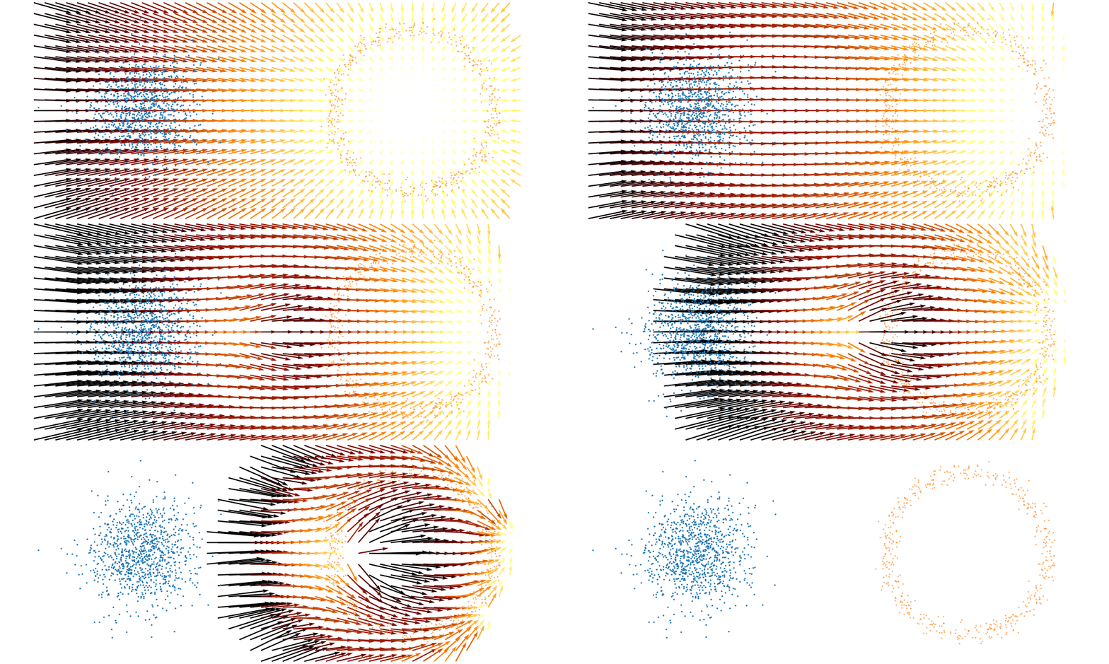
For a visualisation of this you can look at the below figure.

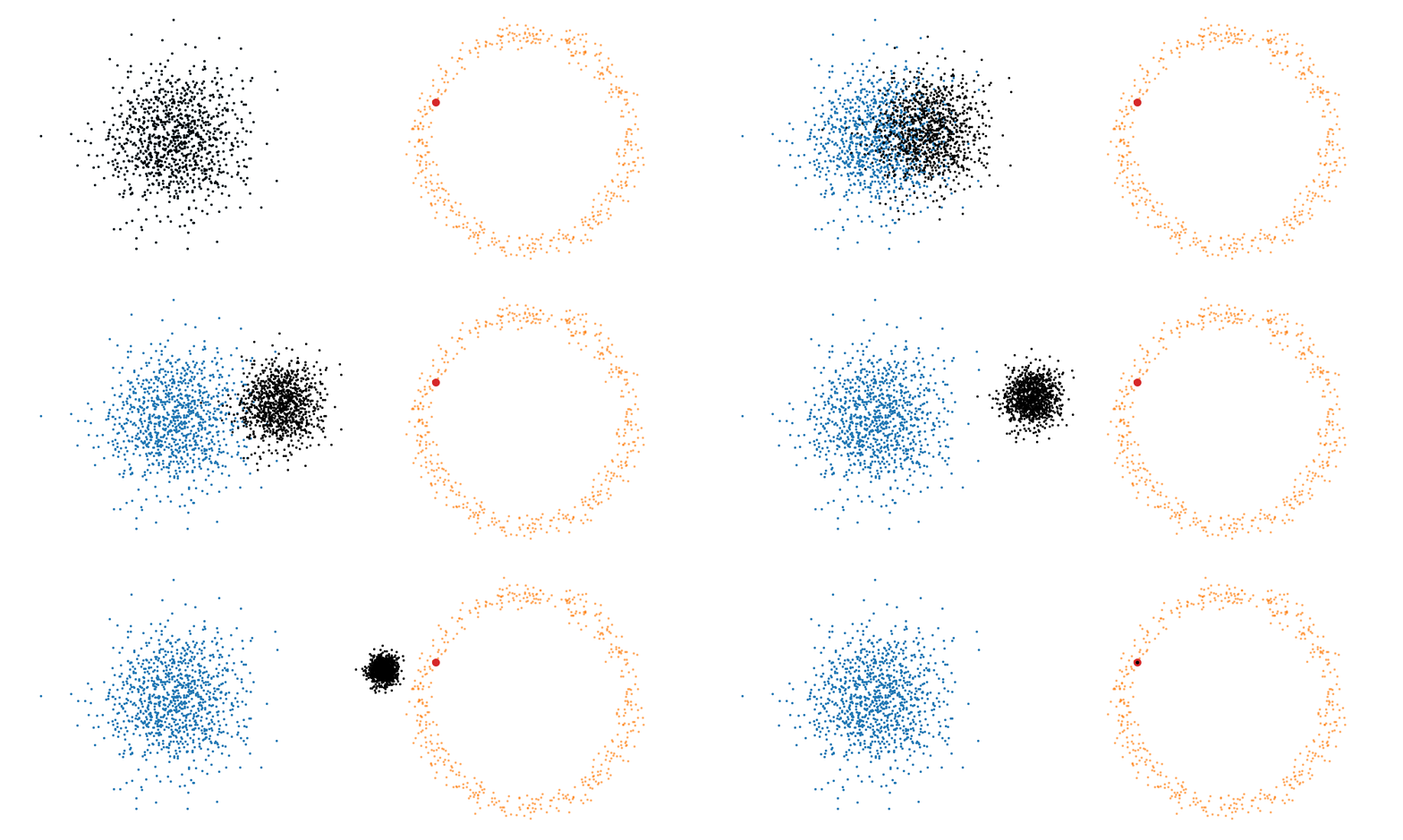
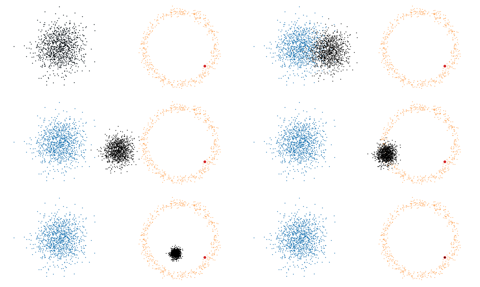
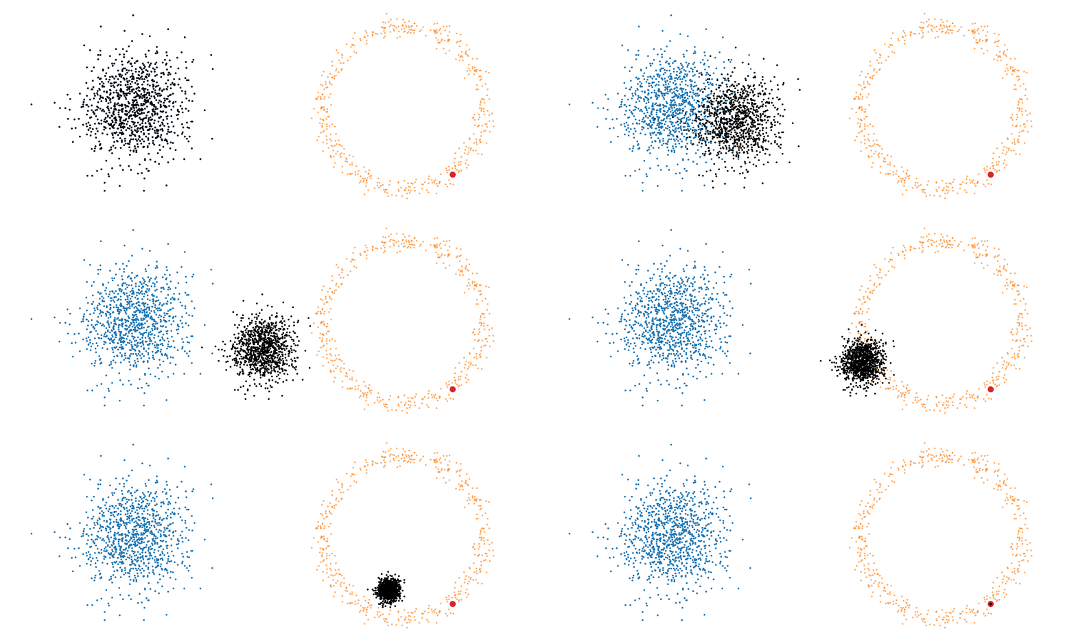
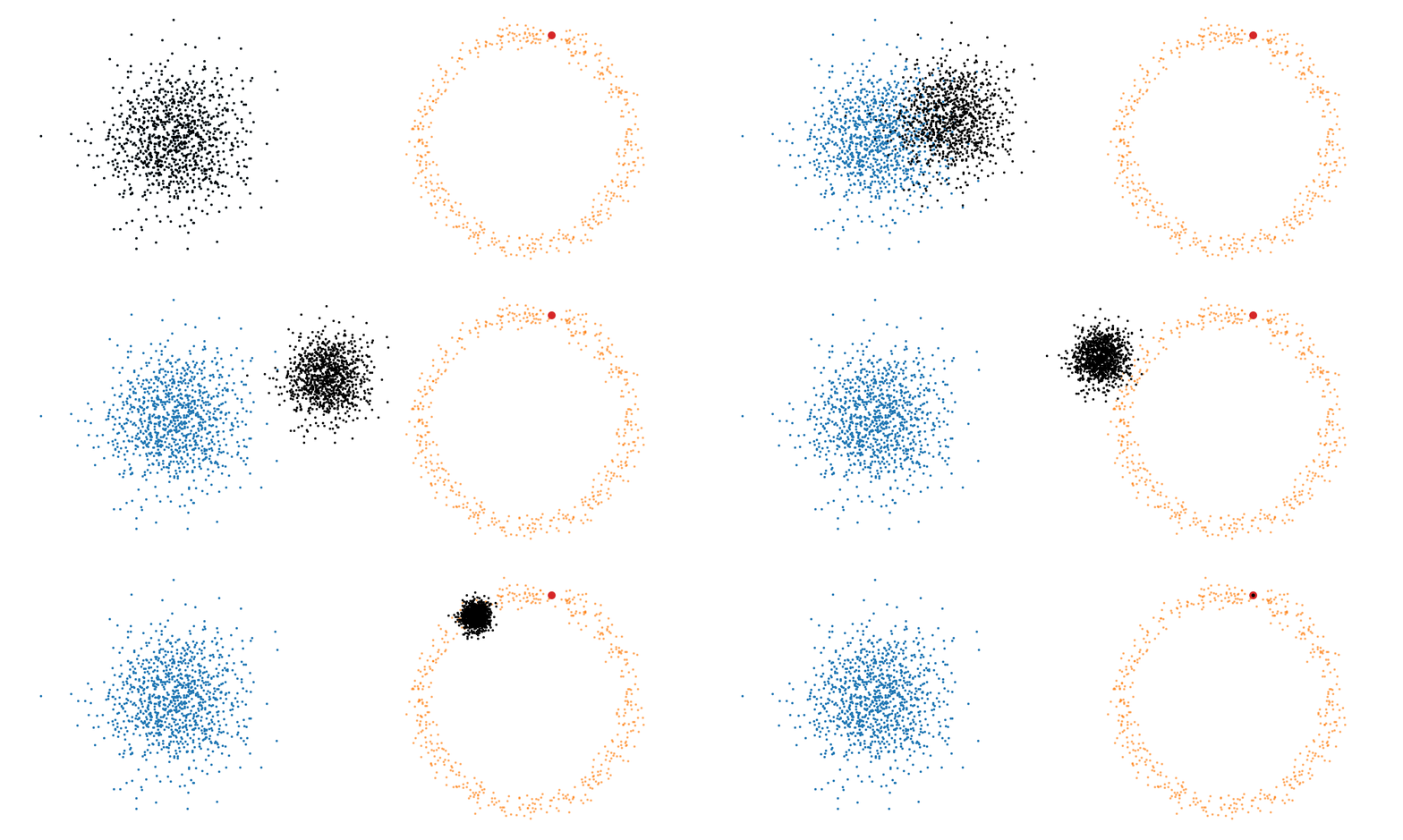
Based on this you can imagine there an underlying vector field which would transport all samples to the given point as shown below.

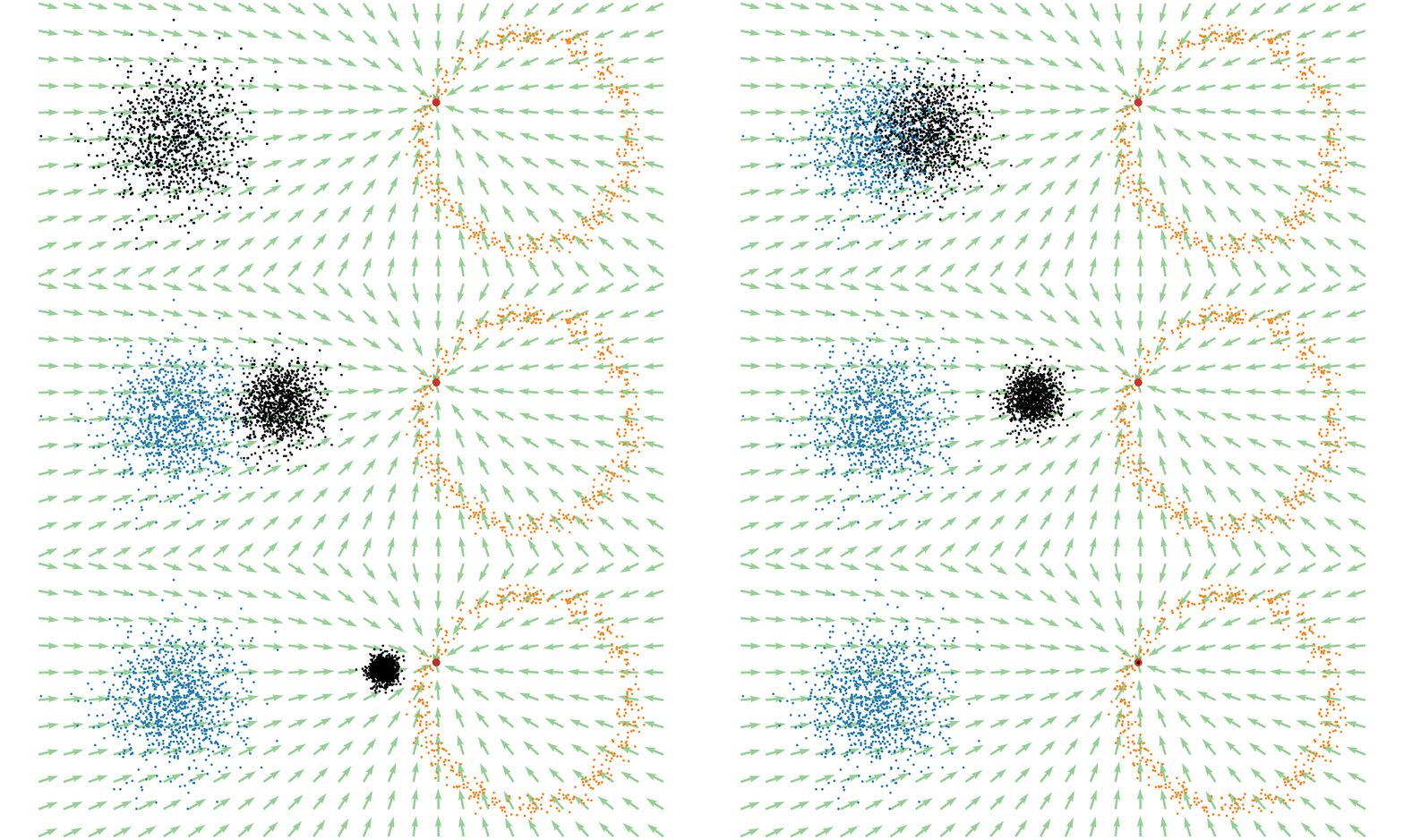
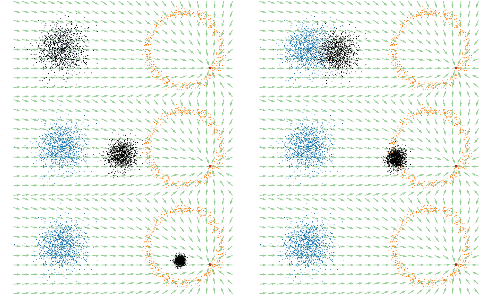
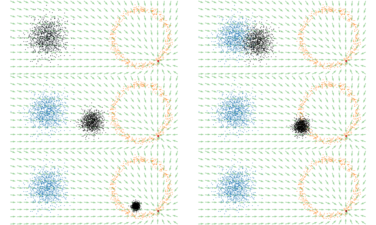
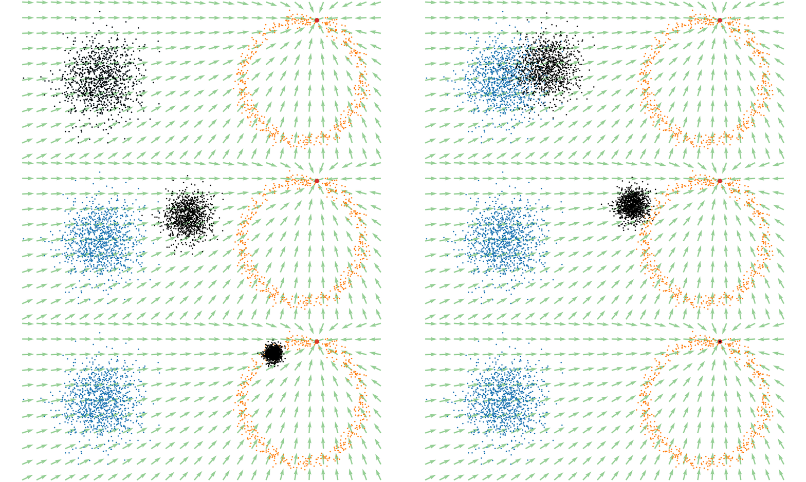
This doesn’t take into account the samples from the base distribution however, so if we want to investigate this directly we would image the path that all the samples would have to take to go from the base distribution to the give sample.

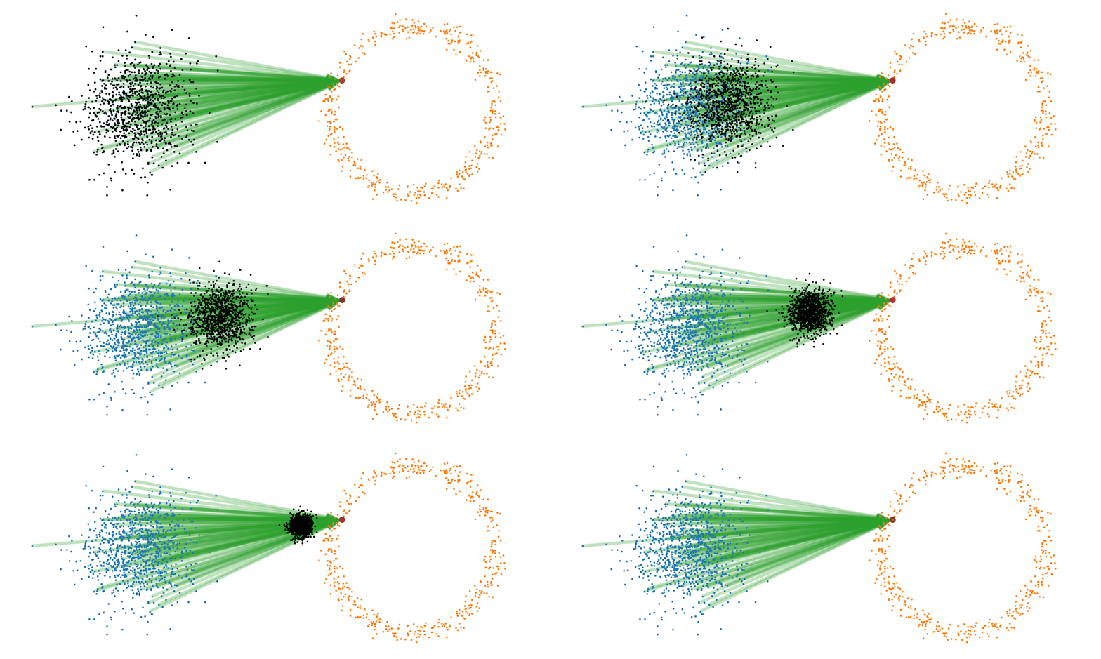
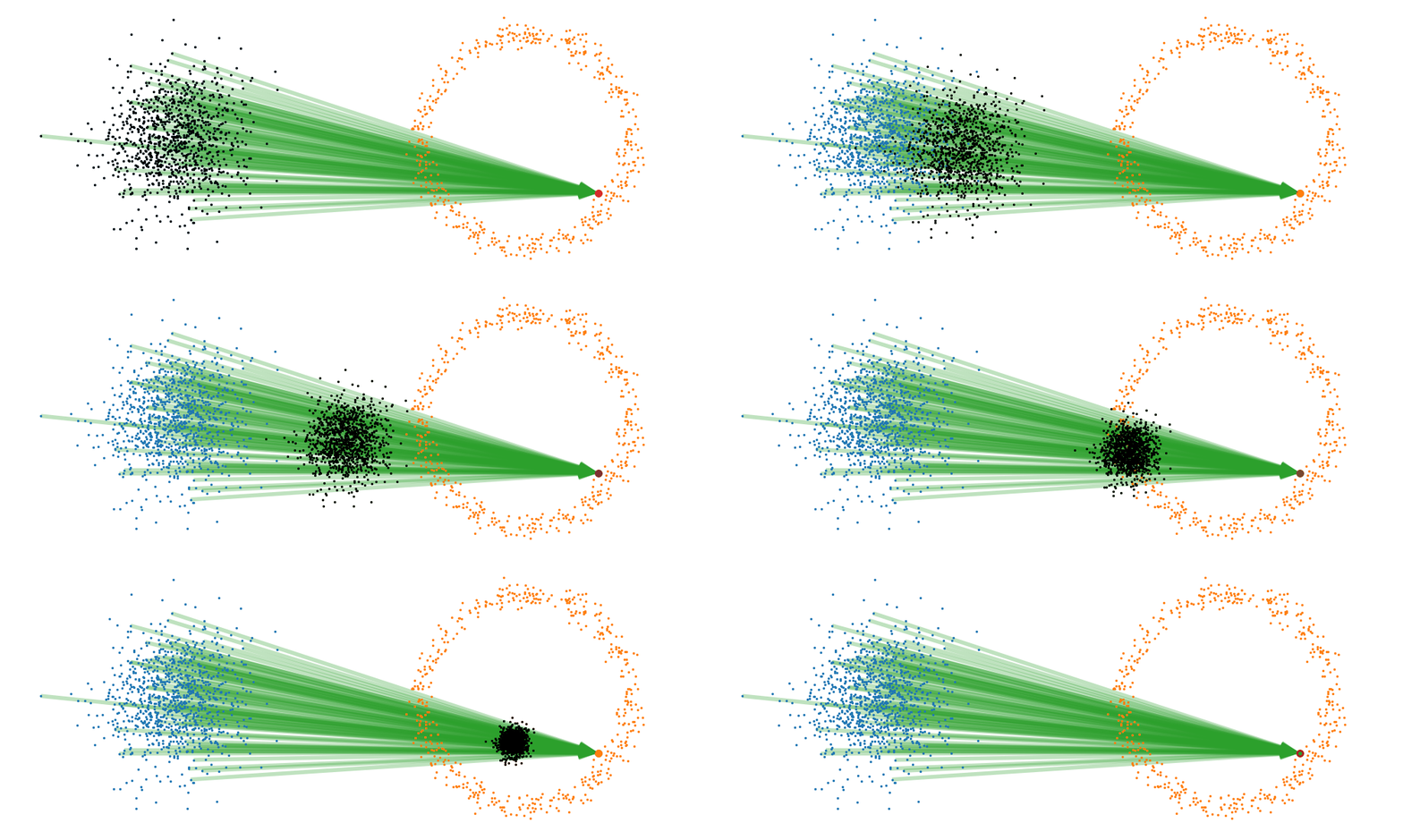
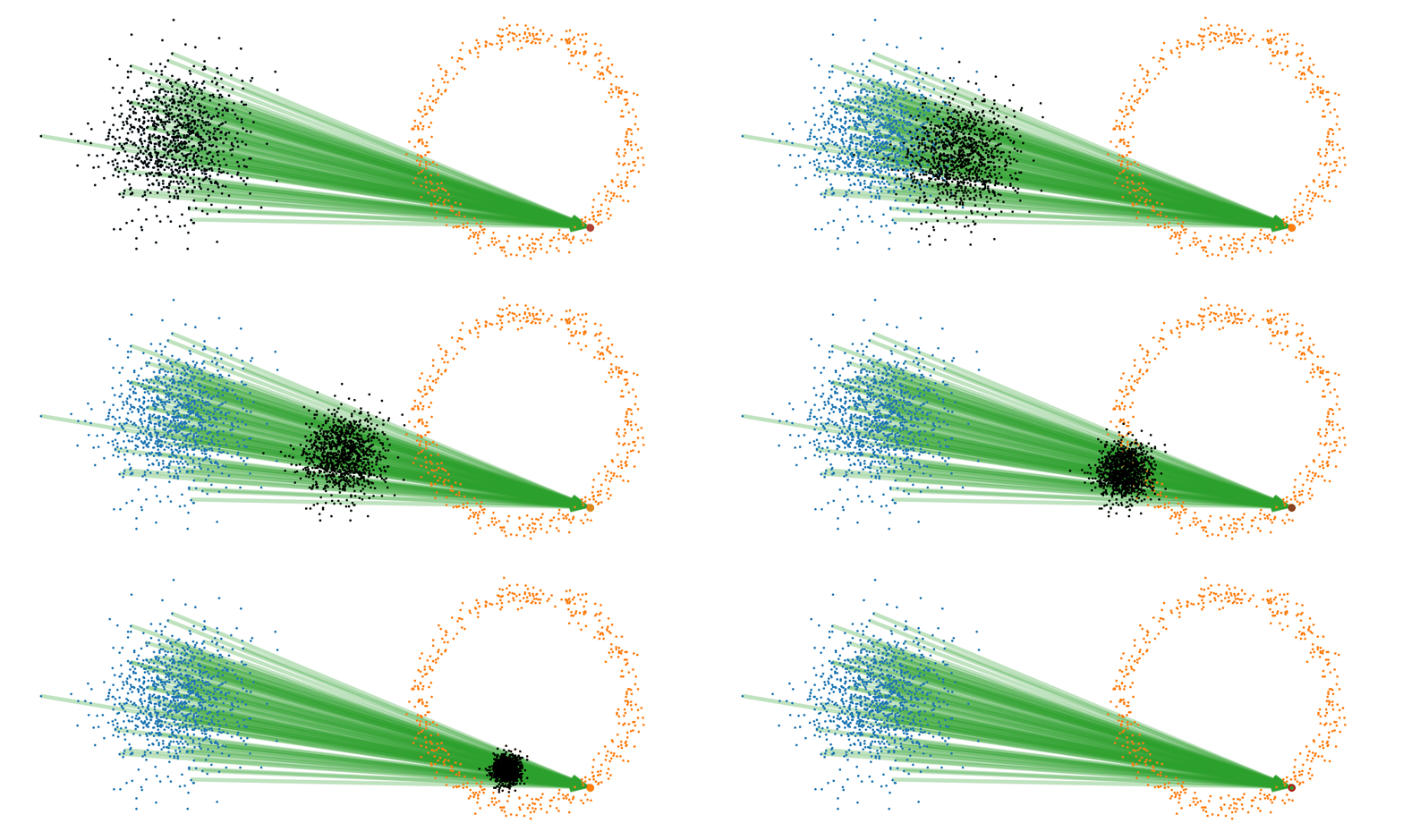
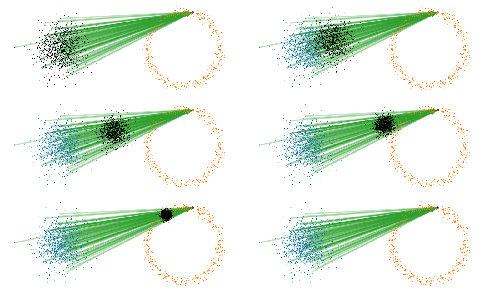
If we then image that each timestep has a given probability if we imagine the first distribution to be known, let’s assume it’s a gaussian for now, then we can create what is called a probability path…

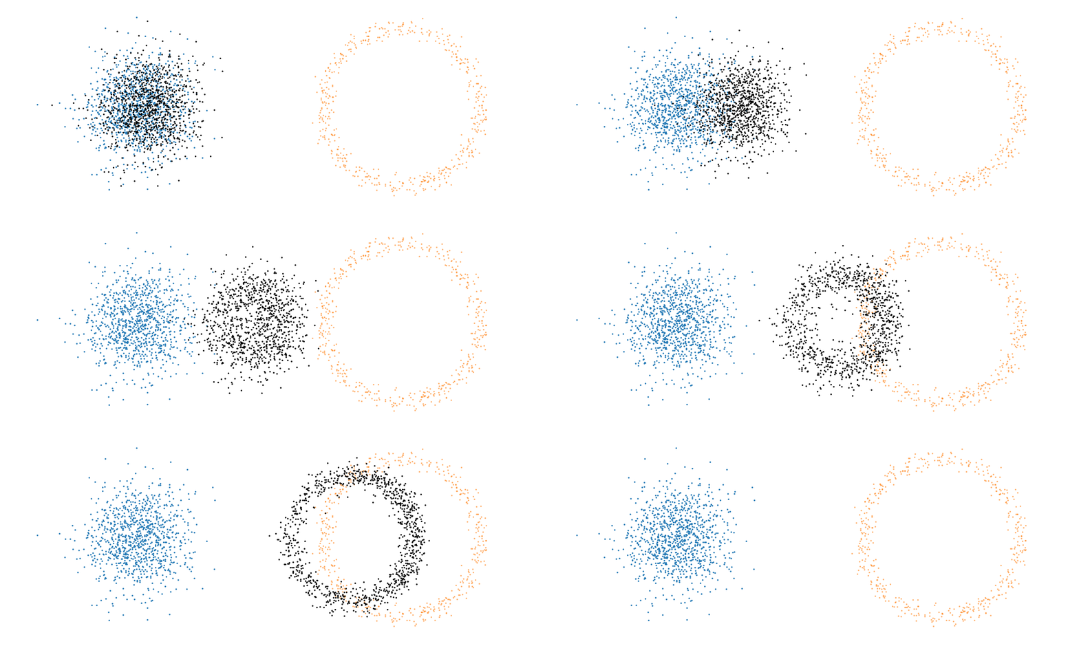
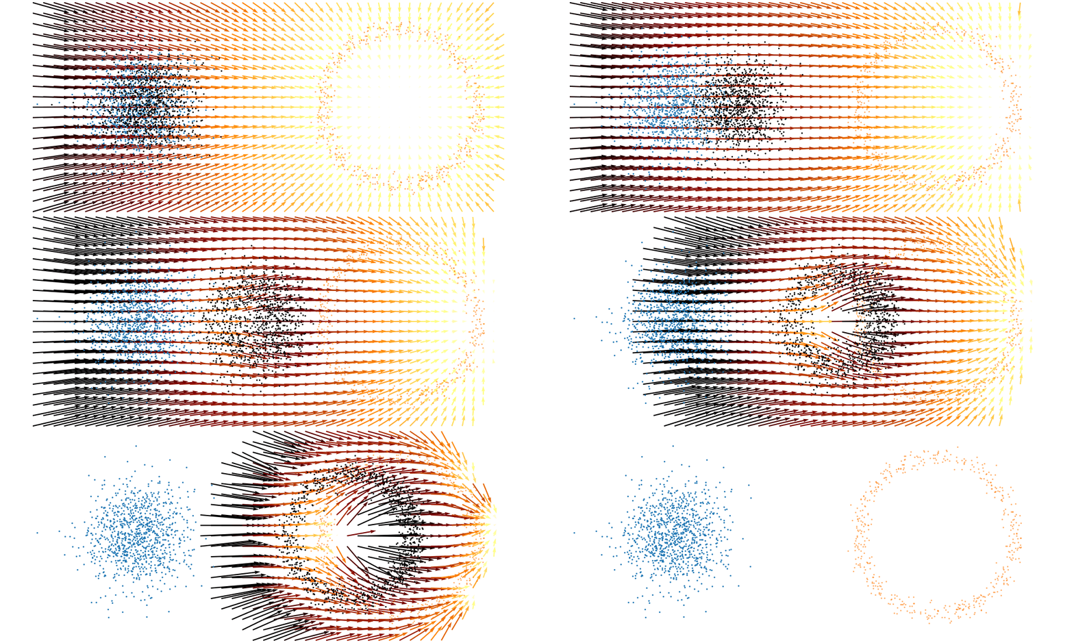
And here’s one I prepared earlier.

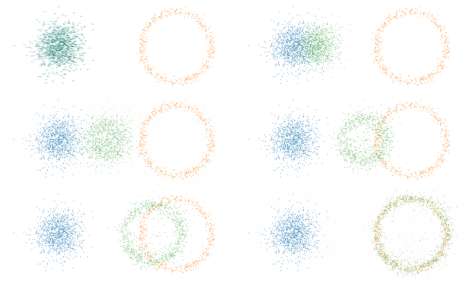
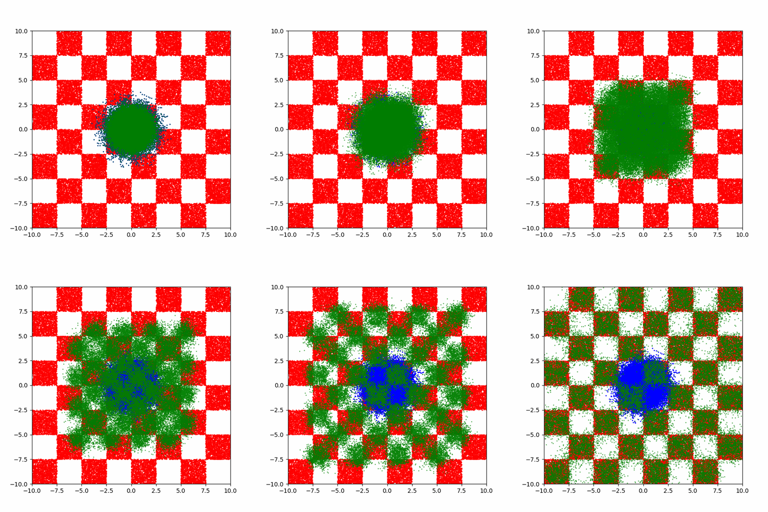
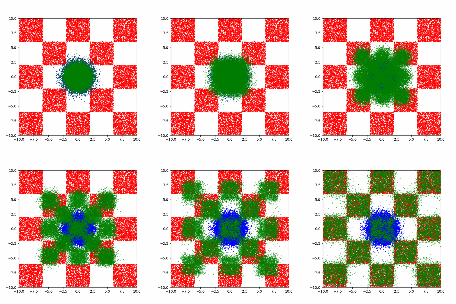
Checkerboard density: Dimensionality and modal scaling behaviour

An example of what this looks like is then below.

Generating MNIST-like images

Conclusion