In this post, I’ll give an introduction to variational autoencoders, with some machine learning examples.

Resources

As usual, here are some of the resources I’m using as references for this post. Feel free to explore them directly if you want more information or if my explanations don’t quite click for you.

• Stanford CS229: Machine Learning | Summer 2019 | Lecture 20 - Variational Autoencoder
• An Introduction to Variational Autoencoders - Diederik P. Kingma, Max Welling
• Variational Autoencoders - Arxiv Insights
• From Autoencoder to Beta-VAE - Lilian Weng
  • Found this after I started making this blog post, it’s basically exactly what I wanted to do theory-wise and more. I’m going to focus a little more on implementation but otherwise I’d recommend going over there if you want extensions to the theory.
• GANs, AEs, and VAEs - Andy Casey
• Understanding Variational Autoencoders (VAEs) | Deep Learning - DeepBean
• Deriving the KL divergence loss in variational autoencoders - Kevin Frans
• Learning Structured Output Representation using Deep Conditional Generative Models
• Conditional Variational Autoencoder for Learned Image

Table of Contents

• Motivation/Traditional Autoencoders
• Core Idea
• Construction of the Loss
• Conclusion

Motivation/Traditional Autoencoders

A big thing in computer science is data compression. Taking high dimensional or simply large unlabelled inputs and reducing their size into some representation that is later interpretable or able to be used as input to reconstruct the original inputs. One particularly successful approach was the Autoencoder, machine learning architecture made up of two neural networks, an encoder that would taken the large input and reduce it into some small latent representation and a decoder that would take the values in this latent distribution and reconstruct the original inputs. The general structure is shown below.

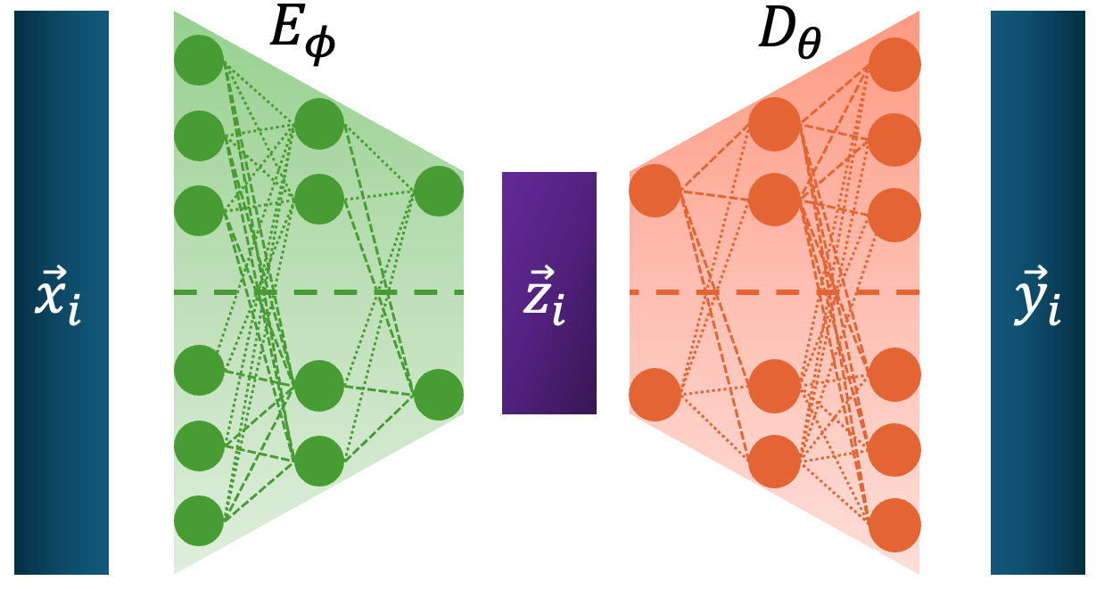
Where \(\vec{z}_i \in \mathbb{R}^K\) is the compressed latent representation for the \(i^{th}\) data point \(\vec{x}_i \in \mathbb{R}^D\) (\(K<<D\)), \(E_\phi\) is the encoder and \(D_\theta\) is the decoder. The loss is then simplify how well the output matches the input, as all we care about is whether a good output can come from the latent vector or ‘bottleneck’. If we just use the L2 norm, for a single datapoint \(\vec{x}_i\) this looks like,

And then for a whole dataset we can either take the sum or average, they’re equivalent up to a multiplicative constant so I’ll just use an average over the data space. For \(M\) datapoints this looks like,

And that’s really it. Very simple but it can do quite a lot. Coding that up real quick this is what it looks like.

class Encoder(nn.Module):
    
    def __init__(self, input_dim, hidden_dim, latent_dim):
        super(Encoder, self).__init__()

        self.layer_1 = nn.Linear(input_dim, hidden_dim)
        self.layer_2 = nn.Linear(hidden_dim, hidden_dim)
        self.layer_3 = nn.Linear(hidden_dim, hidden_dim)
        self.layer_4  = nn.Linear(hidden_dim, latent_dim)
                        
    def forward(self, x_inp):
        x_int       = F.relu(self.layer_1(x_inp))
        x_int       = F.relu(self.layer_2(x_int))
        x_int       = F.relu(self.layer_3(x_int))
        # It's not common to have a sigmoid here, but it makes the plotting later on easier and doesn't change the salient features of the model
        x_int       = torch.sigmoid((self.layer_4(x_int))) 
        
        return x_int


class Decoder(nn.Module):
    def __init__(self, latent_dim, hidden_dim, output_dim):
        super(Decoder, self).__init__()
        self.layer_1 = nn.Linear(latent_dim, hidden_dim)
        self.layer_2 = nn.Linear(hidden_dim, hidden_dim)
        self.layer_3 = nn.Linear(hidden_dim, hidden_dim)
        self.layer_4 = nn.Linear(hidden_dim, output_dim)
        
        
    def forward(self, x_inp):
        x_int     = F.relu(self.layer_1(x_inp))
        x_int     = F.relu(self.layer_2(x_int))
        x_int     = F.relu(self.layer_3(x_int))
        x_hat = torch.sigmoid(self.layer_4(x_int))
        return x_hat


class AEModel(nn.Module):
    def __init__(self, input_dim, latent_dim, encoder_hidden_size, decoder_hidden_size):
        super(AEModel, self).__init__()
        self.E_encoder = Encoder(input_dim=input_dim,    hidden_dim=encoder_hidden_size, latent_dim=latent_dim)
        self.D_decoder = Decoder(latent_dim=latent_dim, hidden_dim = decoder_hidden_size, output_dim = input_dim)
                
                
    def forward(self, x):
        z       = self.E_encoder(x)
        x_hat   = self.D_decoder(z)
        
        return x_hat, z

One of the best ways we can see how well it did is to simply see if it can reproduce the inputs for a testing dataset. In the following I trained on the MNIST dataset comprising of a bunch of handwritten numbers that looks like the below.

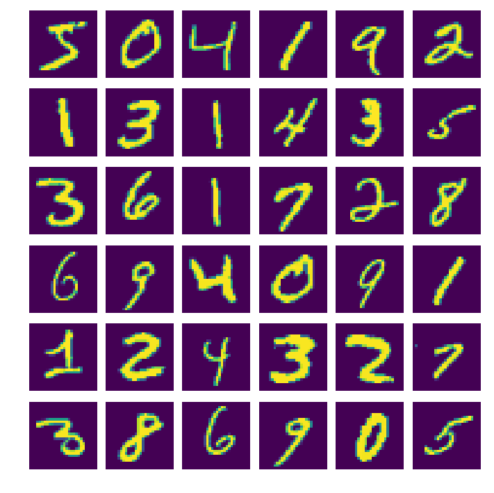
We can train the autoencoder above with \(2\) the number of latent dimensions equal to \(2\) and the number of inputs dimensions of \(28^2\) as the images are \(28\times28\). We can then look at how weel the model does with a few grabs of inputs and outputs.

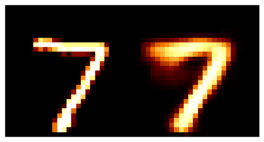
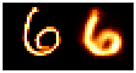
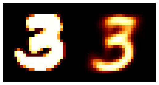
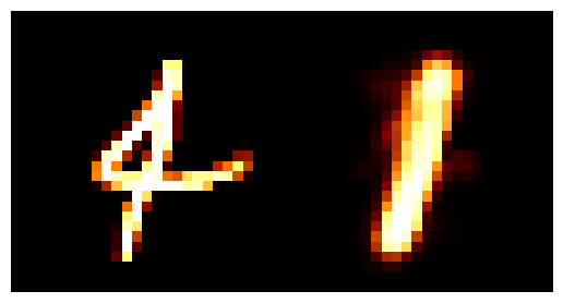
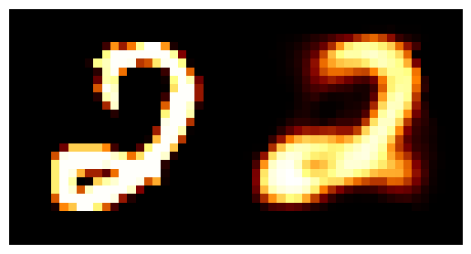
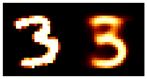
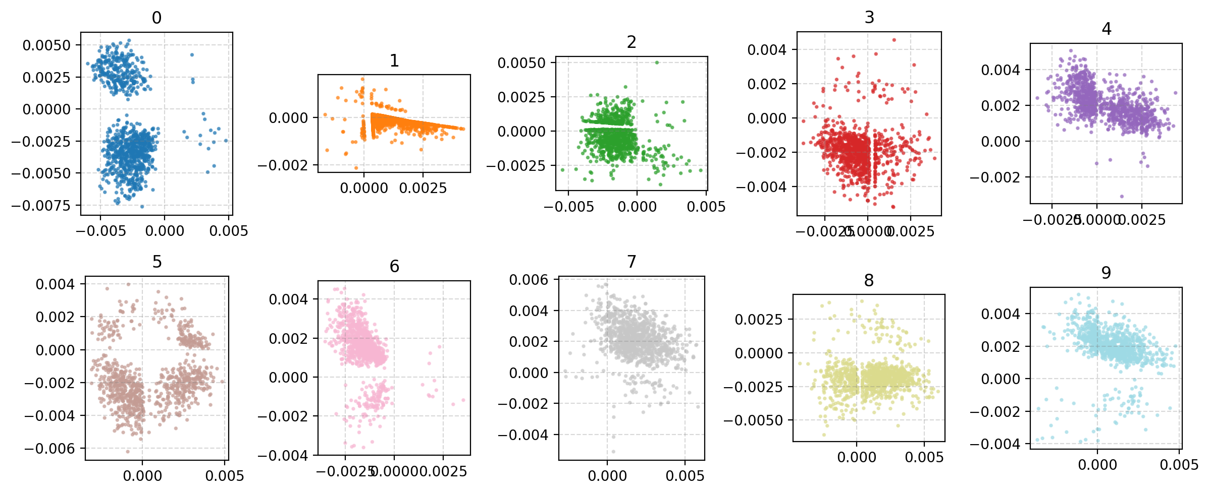
You may be wondering why the post isn’t just on autoencoders as this doesn’t look too bad? Well the issue is more obvious when we investigate the latent space of the model. First let’s see where images in the MNIST dataset land in the latent space (which remember is 2D so we can plot it like this).

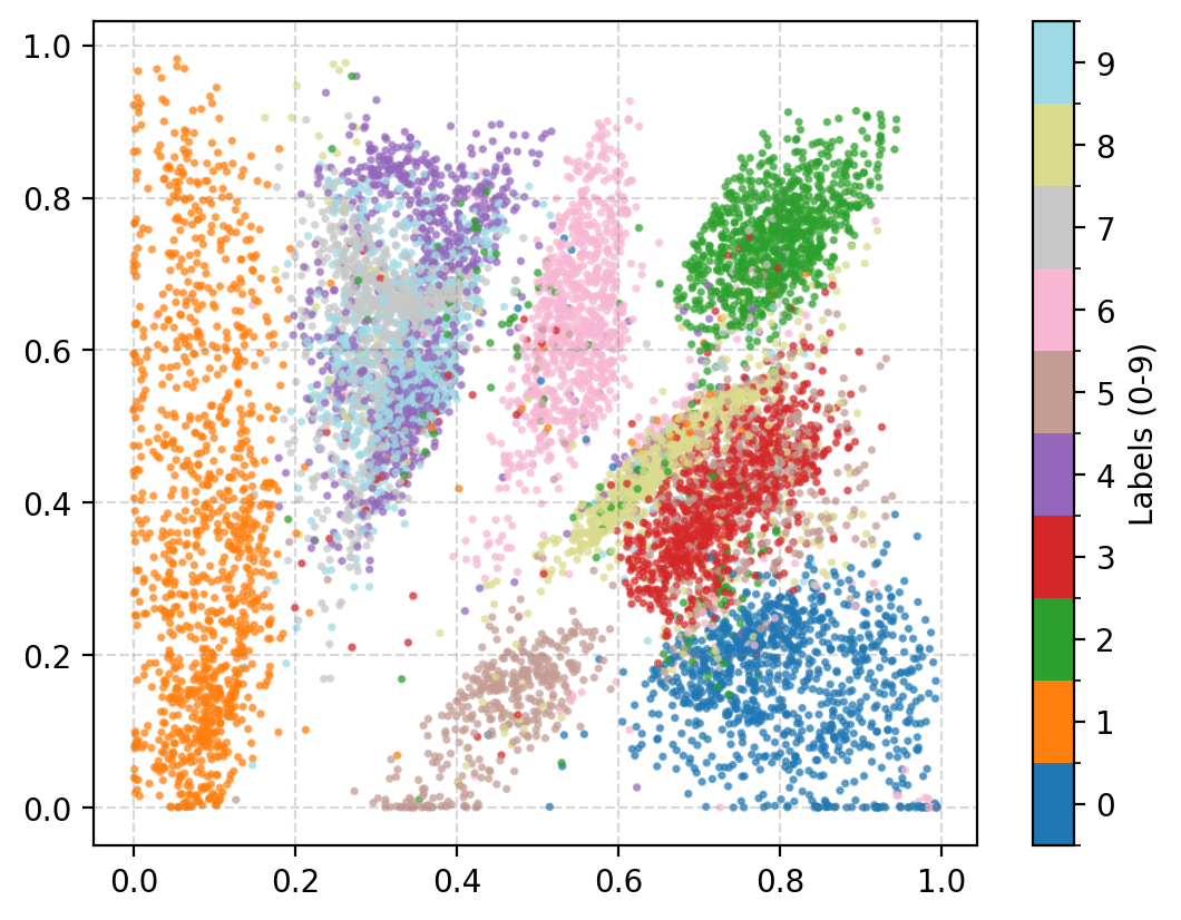
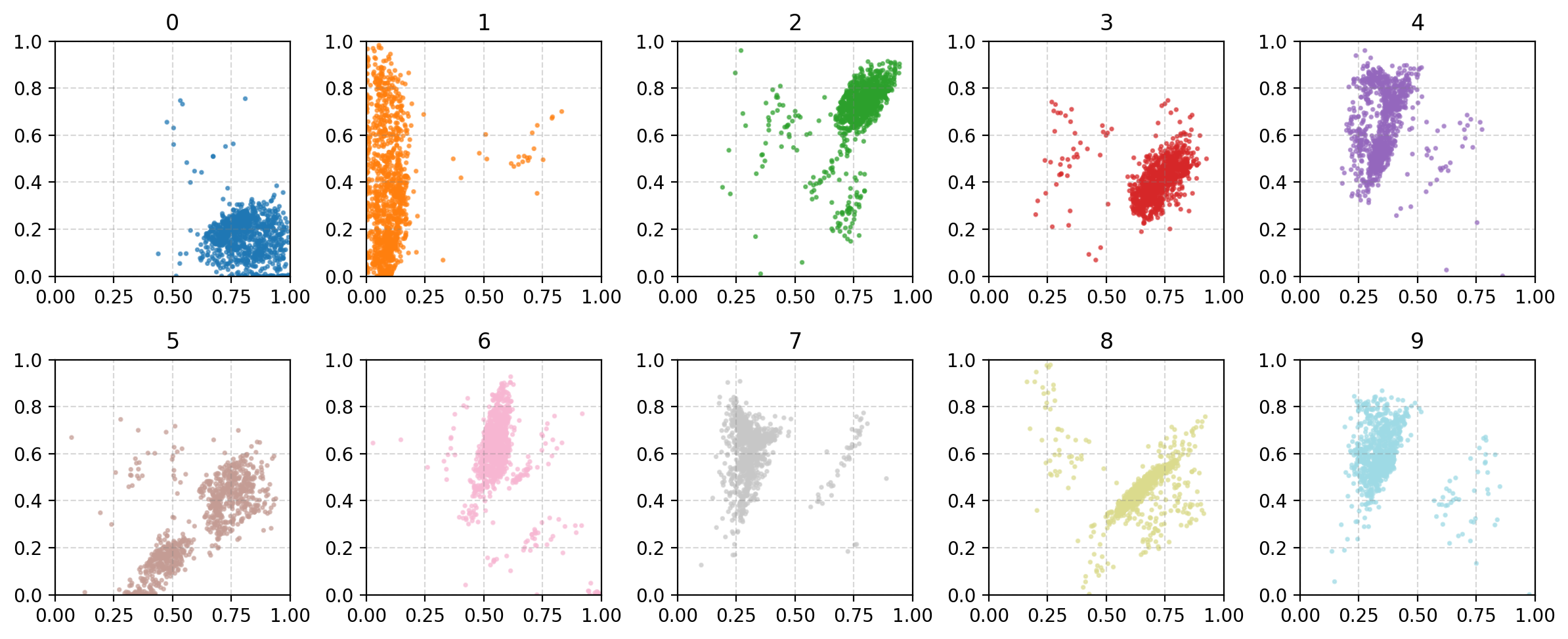
A few things to note:

1. Most of the distributions are bimodal with some parts mapped to one area of the parameter space and others to completely different areas
2. Many of the numbers are overlapping in parameter space, and they don’t even necessarily look similar. (e.g. observe 4, 7 and 9)
3. Numbers that you would think are similar are not necessarily put together (e.g. I would put 0, 9 and 6 together but instead 0 and 3 are close?)
4. There’s areas of the parameter space that are empty, what do these values map to?

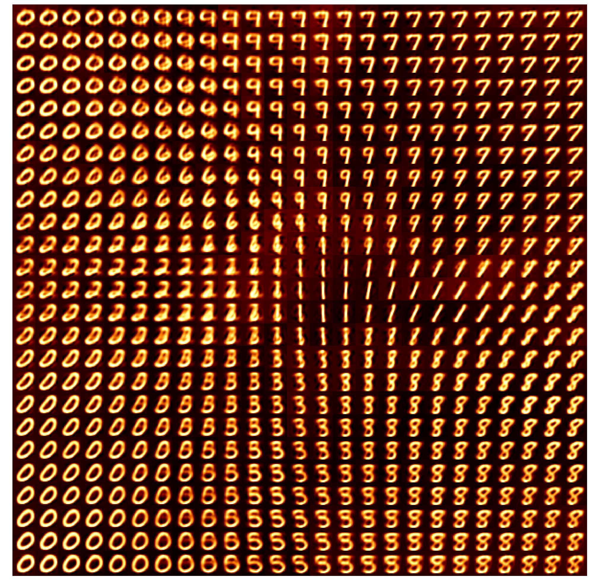
This is effectively looking at how the encoder is understanding the information and the key point is that the latent space is not well structured. We can also see how the space is interpreted by the decoder. Taking in inputs ranging from 0 to 1 in each dimension and seeing what the produce in the data space.

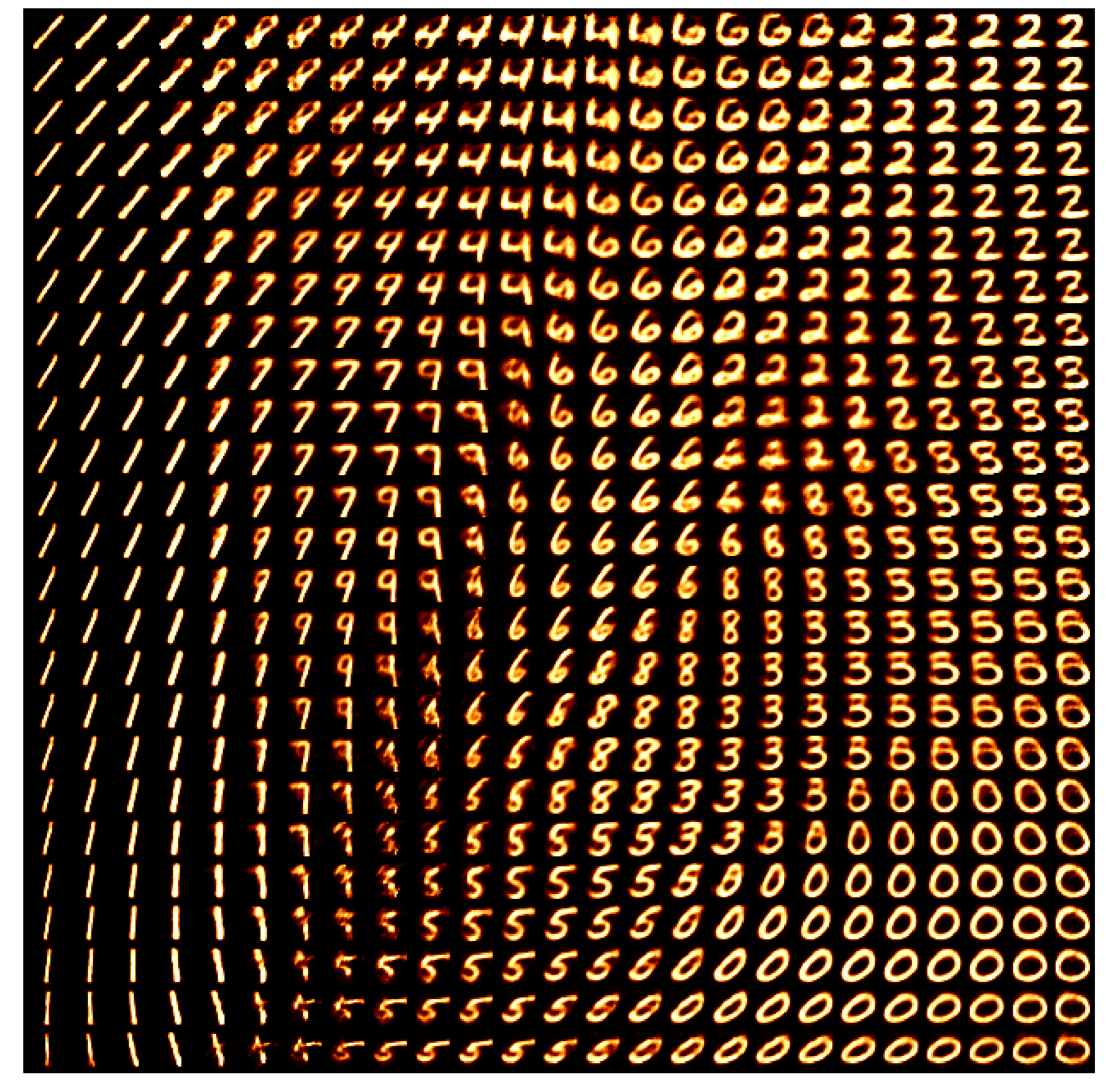
We can now kind of see what’s happening, the autoencoder isn’t mapping numbers that are similarly shaped together. It seems to merely be assigning the numbers areas, and then just phasing between the two with the stages of the phase not corresponding to anything interpretable. e.g. Looking at how the 0 phases into the 5, the ‘inbetween’ doesn’t look like anything that a human would write. You can also clearly see how the ‘5’s show up in two entirely separate areas where if you go between them you get a ‘3’?? Because of this arbitrary assignment the spaces in between numbers that actually populate the space are not interpretable, we can’t say that they will look close to numbers close in the parameter space, it might just be some gobbledygook.

We need some way to essentially make the space more structured. And we can do this by instead of interpreting numbers going to points, mapping them to distributions and saying that they are a draw of said distribution. Implicitly, this also makes the space continuous and allows us to generate “new” data as we can sample these distributions to generate new and possibly realistic data. This is essentially a Variational Autoencoder.

VAE Core Idea

A Variational Autoencoder¹ or VAE has a similar structure to a traditional autoencoder in that it reduces the size of some input, maps this to some latent space, and then maps this back into the data space. The key difference is that the encoder instead of learning the map to the latent space directly, learns the map \(E_\phi\) of the inputs to the parameters that dictate the conditinoal distribution \(p_\phi(\vec{z}_i\vert\vec{x}_i)\). And the decoder \(D_\theta\) then learns the map to the parameters of the conditional distribution of the data given the latent parameters \(q_\theta(\vec{x}_i\vert\vec{z}_i)\). This is shown in the diagram below in the case of both \(p\) and \(q\) being normal distributions.

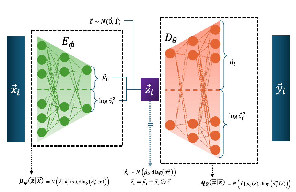
Infuriatingly, for the decoder, it is common to fix the covariance values as it makes the training more difficult. And since the decoder distribution is often a normal the loss eventually turns into the mean squared error, and then they call it the reconstruction loss. So the decoder loses it’s probabilistic interpretation and then some PhD student spends a couple hours trying to figure out why papers still refer to it as a probability distribution only to learn this fun fact at the end… anyways.

And before I move on, just another clarification about the diagram above.

You’ll note that there is an extra input \(\vec{\varepsilon}\) leading into \(\vec{z}_i\). Because we are describing a probability distribution and not some deterministic transformation a particular \(\vec{z}_i\) doesn’t come out of a particular \(\vec{x}_i\) but a particular \(q_\phi(\vec{z}\vert\vec{x}_i)\).

To get a specific \(\vec{z}_i\) for a given \(\vec{x}_i\) we need to sample the given probability distribution \(q_\phi(\vec{z}\vert\vec{x}_i)\). And because the eventual derivatives (which I’m just about to discuss) would be complicated otherwise, we perform the reparameterisation trick.

In case of a normal distribution,

you can off-load the stochasticity of the sampling from the distribution itself to some other variable,

and dilate the distribution by the covariance,

and shift it so that it matches the wanted distribution,

Construction of the loss

Disregarding any level of physical interpretability to \(\vec{z}\) all we care about is how well we can reproduce \(\vec{x}\), or find the parameters \(\phi^*\) and \(\theta^*\) that maximise the probability of our data for the probability distribution,

which can also be expressed as the fully marginalised likelihood (hence why it uses the \(p\) above),

(The following is partly reproducing Equations 2.5-2.9 in 1906.02691 partly adding my own spin.)

This is the evidence and a little hard to calculate, additionally, in practice we want to average over the samples from our latent distribution. So we’ll average over these samples, which is over \(\vec{z}_i\) which theoretically isn’t doing anything as the evidence doesn’t take this as input,

and then use Bayes’ theorem and a little algebraic trickery to split it into some more managable parts,

And now we also meaningfully introduced \(q_\phi(\vec{z}\vert\vec{x})\) that has \(\phi\) in it! And if you’re familiar with variational inference (if here’s a quick plug for my post on that) this may look familiar as the following.

We can then see that,

which indicates that if we maximise the ELBO then we concurrently maximise the evidence and minimise the KL divergence (something akin to the distance between the posteriors that \(q_\phi\) and indirectly \(p_\theta\) describe which should be the same thing). We can still split this into a more telligible form.

Now we can clearly see that in the first term we are trying to minimise the distance between what is our approximate posterior and assumed prior, a kind of regularisation term saying to not go to far away from the prior and do something crazy, and the second term is straight reconstruction accuracy, for the given \(x\)s, we want to maximise the likelihood/how well the sampled likelihood is reproducing the input data.

In the case where the VAE is learning the parameters of a normal distribution instead of calculating the regularisation term numerical, we can do a quick bit of algebra to get it in an algebraic form. With the following,

which because we’re assuming that we’re modelling a uncorrelated gaussian/the pixels in the MNIST data are independent, the log of this simplifies to,

Where \(j\) is indexing a given dimension of \(\vec{z}\), not a datapoint. Additionally, assuming that the prior \(p(z)\) is a uncorrelated standard normal distribution (unit variance) centred at \(\vec{0}\) we can similarly express it’s log as the following,

And then combining the two within the KL divergence,

Then we’re going to be a little sneaky and not that these samples are explicitly about the “true” posterior, but our approximate distribution. So the mean and variance of the samples that the averages are taken with respect to are the average and mean parameters of our approximate distribution. This allows us to simplify the two averages as the following.

So that sorts out our KL divergence, but we still need to calculate our reconstruction loss. Thankfully we already contructed everything with the reparmeterisation trick so we can perform backwards propagation, but for any given input we only sample \(\vec{z}\) once (let’s denote this \(\vec{z}'\)) so we can’t properly perform Monte Carlo integration / numerically calculate the average. Well it actually practically turns out fine I believe in part because this training is done over multiple iterations and so you sample a range of random samples \(\vec{\varepsilon}\) over the course of training and the final result is relatively stable. I think of it adding a little extra stochasticity to the gradient descent (whether it is something like ADAM or already SGD).

So, the TLDR is that our loss now looks like the following,

And then as stated above, for numerical stability issues the covariance/standard deviations \(\sigma_n^{\{p\}}\) of \(p_\theta\) are often fixed to 1 which simplifies this further (adding superscripts to now denote the different distributions the means and standard deviations come from) while throwing away the constants

MNIST with VAE

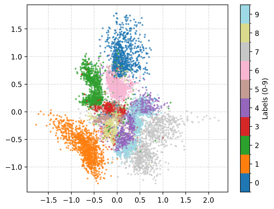
Let’s see how the above performs on the same MNIST data we had before. Using the same kind of diagnostic figures we see.

First we’ll look at how the training data maps into the latent space of the VAE.

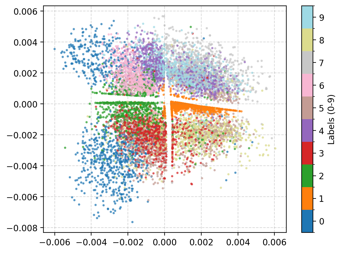
There’s definitely more defined structure there with more similarly shaped numbers put close to each other and less areas where numbers are mapped to that are distinct to the others. We want a continuous probability of grouping where the probability of something that is a 0 should feasibly have a reasonable chance of being a 9.

Looking at the latent space directly we can then see the following.

On the surface this seems to have a similar quality to the autoencoder version but notice that the transitions between numbers makes more sense more often here like the 3/5/8 area on the bottom right or the 0->9->7 on the top.

Another benefit that I couldn’t really show was that the VAE results it took a lot less hyperparameter tuning. I chose some simple neural networks and fiddled with the learning rate a little and then got the results above. With the relevant autoencoder results, I had to trial and error batch sizes, learning rates, number of network layers, number of network nodes and probably fought against my own point because the autoencoder results on the surface don’t look to bad.

Another thing that isn’t necessarily working in my favour is that we chose a normal distribution for the likelihood distribution/decoder. The data here is ranging from 0 to 1 so it might make more sense to choose some constrained distribution instead such as a Beta or Binomial distribution. In the case of the binomial distribution the reproduction loss becomes a binary cross entropy but is otherwise much the same. (and we simultaneously get around some inherent numerical instability issues involving the use of the MSE).

Using that we get the following.

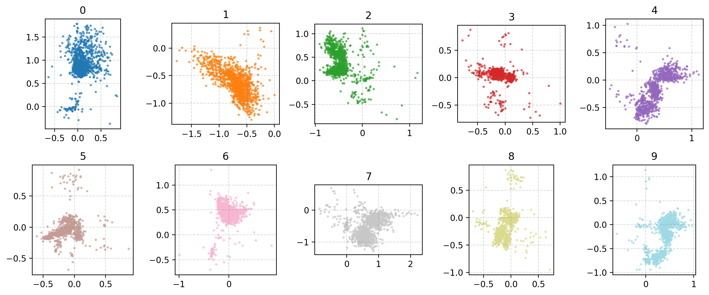
And.

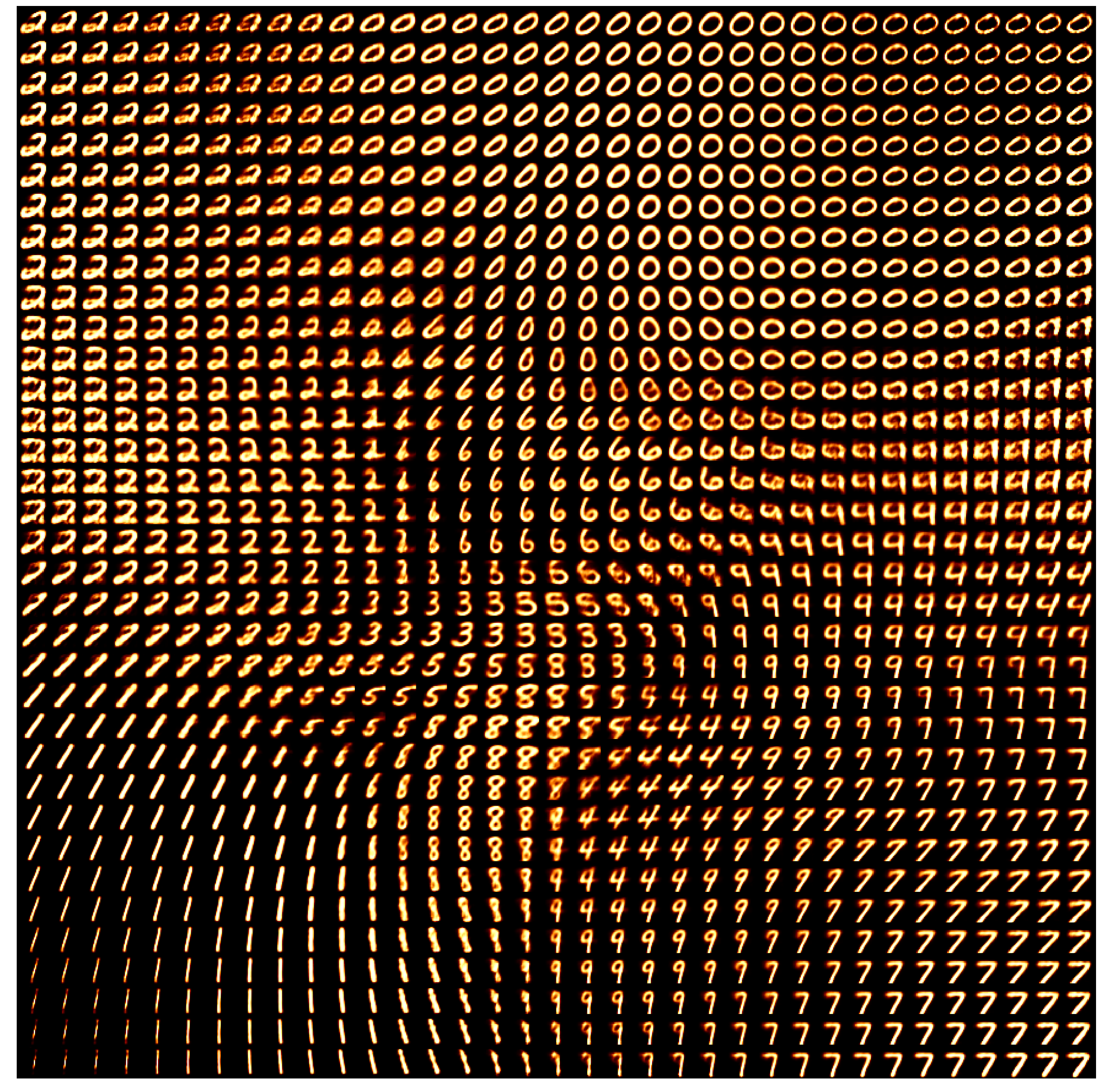
You can see that we get less of the background colour than we do with the normal distribution likelihood and the numbers themselves are also clearer.

Conclusion

Variational autoencoders as I’ve shown above are basically old ideas now (see Lilian Wang’s post for some of the stuff they were doing it just in 2019) but are foundational to how many people thing of data encoding and many modern architectures that I’ve seen incorporate some variant of a VAE precisely for data reduction. For example neural posterior estimation using normalising flows still often use some form of encoder structure for data embeddings where they create a lower dimensional summary of the data to feed into the normalising flow transformations (see my post on it if you wanna learn more). So I hope you had a nice time learning about VAE’s and if you have any comments or suggestions please send them to [myfname.mylname]@monash.edu.

Black Box VI with CVAE

I originally also wanted to show how one could then perform variational inference or SBI with conditional variational autoencoders (or here for another ref) but had already spent too much time on the above. May revisit later on so stay tuned.