In this post, I’ll attempt to give an introduction to simulation-based inference specifically delving into the method of NRE including rudimentary implementations. UNDER CONSTRUCTION

Resources

As usual, here are some of the resources I’m using as references for this post. Feel free to explore them directly if you want more information or if my explanations don’t quite click for you. I will highly recommend it for this particular post as I’m using it as motivation to learn about these methods myself in more detail.

• A robust neural determination of the source-count distribution of the Fermi-LAT sky at high latitudes by Eckner et al.
• The frontier of simulation-based inference by Kyle Cranmer, Johann Brehmer and Gilles Louppe
• Recent Advances in Simulation-based Inference for Gravitational Wave Data Analysis by Bo Liang and He Wang
  • Really recommend giving this a read, it’s hard to find papers that discuss the general topics without getting into the weeds of the specific implementation that they are trying to advocate for or simply too vague.
• Consistency Models for Scalable and Fast Simulation-Based Inference
• Missing data in amortized simulation-based neural posterior estimation
  • Only paper I’ve read that directly and nicely talks about using aggregator networks for variable dataset sizes
• Likelihood-free MCMC with Amortized Approximate Ratio Estimators
  • Specifically sections 2.2 and 3.1
• Contrastive Neural Ratio Estimation for Simulation-based Inference
• LAMPE - Neural Ratio Estimation Tutorial

Table of Contents

• Motivation
• Core Idea
• Neural Ratio Estimation
  • A side note on final layer sigmoid
• Rudimentary Implementations
  • Binary Classifier Network
  • Per Event Level NRE
  • Dataset Level NRE
• Conclusion

Motivation

The TLDR of simulation-based-inference (SBI)¹ is that you have a prior on some parameters \(\vec{\theta}\) and a simulator \(g\), which can give you realistic data \(\vec{x}=g(\vec{\theta})\), and you utilise advances in machine learning to learn the likelihood or posterior for use in analysis without having to actually specify the likelihood directly¹.

The benefits of SBI include but are not limited to:

1. The ability to handle large numbers of nuisance parameters (see above)
2. The user does not have to specify the likelihood and allows direct inference if a realistic simulator already exists (e.g. climate modelling)
3. There have been a few works showing that SBI methods can better handle highly non-gaussian and highly-multi-modal relationships within probability distributions
4. Amortised inference, you can train a model to approximate the probabilities for a dataset and then re-use for other observations relatively trivially
5. Through the use of the simulators and neural networks involved, SBI is generally easier to parallelise
6. Efficient exploration of parameter space, through the fact that the simulator will often only output realistic data, the algorithms don’t have to waste time in regions of the parameter space that don’t lead to realistic data.

The ability to handle a large number of nuisance parameters is actually what sparked my interest in SBI through the paper A robust neural determination of the source-count distribution of the Fermi-LAT sky at high latitudes by Eckner et al. who used Nested Ratio Estimation (a variant of NRE, which I’ll discuss later) to analyse data with a huge number of nuisance parameters introduced by an unknown source distribution in the gamma-ray sky.

I would recommend looking at The frontier of simulation-based inference by Kyle Cranmer, Johann Brehmer and Gilles Louppe and the references therein to check these claims out for yourself if you want.

And more recently, I came across this great paper by Bo Liang and He Wang called Recent Advances in Simulation-based Inference for Gravitational Wave Data Analysis that discusses the use of SBI within gravitational wave data analysis (in the title I know) but it also discusses some of the popular SBI methods in use as of writing. So, I thought I would try and touch on how each of them work in a little more detail than the paper allowed and try to make it a little more general, additionally showing some rudimentary implementations of some of them, with the end goal really being understanding the below figure (Fig. 1 from the paper).

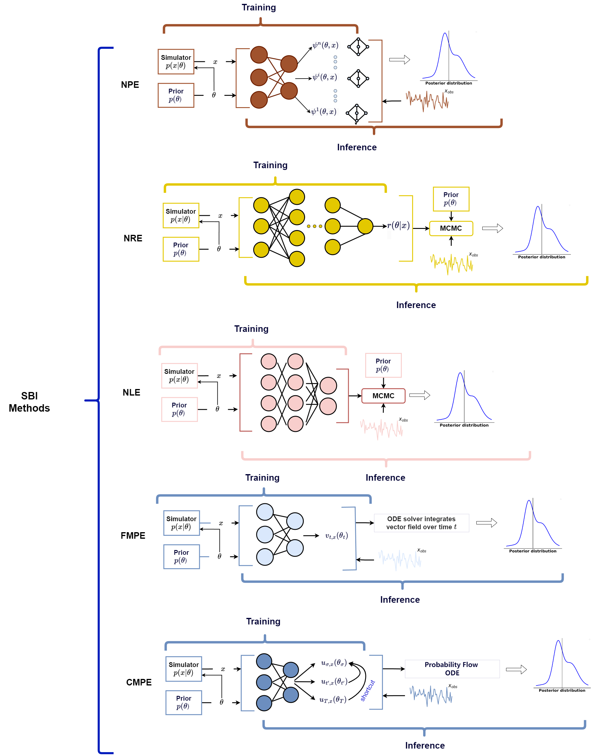
In my last post I went through Neural Posterior Estimation and Neural Likelihood Estimation, and in this post I’ll attempt to go through a basic implmentation of Neural Ratio Estimation and in future posts Classifer-based Mutual Posterior Estimation and finally Flow Matching Posterior Estimation (rough order of how hard it will be to make rudimentary implementations).

Core Idea (Repeat of last post)

First we assume that one has priors for the set of hyperparameters that theoretically influence the data of a given system. e.g.

where \(\vec{\theta}\) is the set of hyperparameters we are interested in. And further assume (for now) that either:

• the set of nuisance parameters \(\vec{\eta}\) can be further sampled based on these values,
• or that the two sets are independent.

Taking the stronger assumption of independence as it is often not restricting in practice,

Denoting the simulator that takes in these values and outputs possible realisations of the data as \(g\) then,

This is in effect samples from the likelihood and with this we have samples from the joint probability distribution through Bayes’ theorem with marginalisation over the nuisance parameters ,

assuming that we can robustly sample over the space of nuisance parameters, we can imagine simultaneously marginalising them out² when generating the samples such that³,

Now because we have these samples, we can try and approximate the various densities that are behind them, using variational approximations such as normalising flows, variational autoencoders, etc. And that’s SBI, the different methods differ in specifically how they choose to model these densities (e.g. flow vs VAE) and importantly which densities they are actually trying to approximate. e.g. Neural Posterior Estimation directly models the posterior density \(p(\vec{\theta}\vert\vec{x})\), while Neural Likelihood Estimation tries to model the likelihood \(\mathcal{L}(\vec{x}\vert \vec{\theta})\) and then you use something like MCMC to obtain the posterior density \(p(\vec{\theta}\vert\vec{x})\).

Something a little different compared to the other methods in the list above, is Neural Ratio Estimation. The TLDR is that you train a binary classifier to distinguish between samples that came from the joint density \(\vec{x}, \vec{\theta} \sim p(\vec{x}, \vec{\theta})\) and those that came from the marginals \(\vec{x}, \vec{\theta} \sim p(\vec{x})p(\vec{\theta})\) or in essence when they are unrelated. Let’s see how that works.

Neural Ratio Estimation

Let’s denote samples that came from the joint distribution as \(y=1\), and those that came from independent marginals as \(y=0\).

We have our samples from the joint distribution, but how do we get samples from the marginals? Well the main characteristic of these samples is that they are unrelated. Presuming that our joint samples are representative, we can sample the same amount again \(\vec{x}_m, \vec{\theta}_m \sim p(\vec{x}, \vec{\theta})\) with a subscript to denote which samples we’re looking at.

Now all that we want is to shuffle these samples, so that the \(\vec{x}_m\) samples have no relation to the \(\vec{\theta}_m\) samples. And by learning when the \(\vec{x}\) is related to \(\vec{\theta}\) we secretly learn the likelihood \(\mathcal{L}(\vec{x}\vert\vec{\theta})\).

The key assumption of this method is that these samples are actually representative enough to make the classifier robust. Presuming that this is the case, then we can say, for some classifier \(f_\varphi\) the optimal solution is that it represents the probability of a sample coming from one distribution or the other⁴. In essence,

We’re now going to do some algebraic manipulation which all we need to remember is Bayes’ theorem,

Doing as such presuming that the prior of a given sample coming from the joint density or the marginals is the same,

Then by constructing we know that,

So,

At this point you might be thinking “whoop-di-doo”, well with one further slight manipulation you can see the benefit.

The likelihood to evidence ratio, and we have the prior used to generate the simulations so by applying that you have a functional form of the posterior.

And \(\vec{x}_i\) does not generally mean they are representing single data ponits, but sets of data corresponding to the hyper-parameters \(\vec{\theta}_i\).

This setup has several benefits including and not limited to the reasons mentioned above and including and not limited to:

• you do not need a functional form of your likelihood (arguably the main reason and similar to the other methods)
• you can construct a likelihood function with gradient support
• the constructed likelihood can be orders of magnitude cheaper to evaluate than an analytical one
• it seems really cool compared to MCMC (joke)

A side note about using Sigmoid

Commonly the final layer of classifiers is a sigmoid function to make the output between 0 and 1,

What amazing about this, is if we chuck in we represent our network up to the final layer before a potential sigmoid as \(\ell\) then our classifer can be expressed as,

and our log-likelihood ratio (which we will later use in training),

i.e. The logit in the final layer of the classifier is our log-likelihood ratio. This, and the fact that naive implements of the sigmoid can cause vanishing gradients/numerical instabilities, motivates us to not have this activation at the end of our network but instead migrate it into the loss. So that we can train the classifier as a classifier but then very easily use it as a log-likelihood ratio!

Rudimentary Implementations

Similar to my previous post we can make the dependencies in the above expression \(\vec{x}\) single data points (as was expressed for the NLE) or for an entire dataset (as was done for NPE). Unlike for those methods, I will show implementations for the per-event likelihood and the dataset level likelihood.

Binary Classifier Network

Before I get into the specifics we will first construct our Binary Classifier Network, as it will be the same for both approaches (the differences will be in how we handle the data in embedding). We’ll leave the number of hidden nodes free and use one hidden layer and leave the dimensionality of the input free for now as well.

import torch.nn as nn
import torch.nn.functional as F

class BinaryNet(nn.Module):
    def __init__(self, input_dim=2, hidden_nodes=16):
        super().__init__()
        self.net = nn.Sequential(
            nn.Linear(input_dim, hidden_nodes),
            nn.ReLU(),
            nn.Linear(hidden_nodes, hidden_nodes),
            nn.ReLU(),
            nn.Linear(hidden_nodes, 1),
            # nn.Sigmoid()
        )
    def forward(self, x):

        # no sigmoid or softmax function here!
        return self.net(x)

And I would like to emphasize that the “\(y\)”s and “\(x\)”s in the code do not necessarily map to anything in the math, its purely to denote ‘input’ and ‘output’.

Per Event Rudimentary Implementation

For a per-event level implementation where the dimensionality of the data is close to that of the hyper-parameters, we can just feed them all into the network without an embedding as I’ve done in other posts (and will go through again in the dataset level implementation). In which case the NRE model is essentially a wrapper for the classifier.

class NRE(nn.Module):
    def __init__(self, data_dim=1, theta_dim=1, hidden_nodes=16):
        super().__init__()
        combined_dims = data_dim + theta_dim

        self.binary_net = BinaryNet(combined_dims, hidden_nodes=hidden_nodes)


    def forward(self, data, theta):
        # assuming that the input shapes are (batch_dim, data/theta dim)
        combined_dataset = torch.concat((data, theta), dim=1)

        return self.binary_net(combined_dataset)

And we’re done! That’s really it. Now we need something to test our model with. I’m going to keep it simple and fit for a single hyper-parameter that dictates the centre of some 2D gaussian with fixed with. We can initialise our model already as we just require the dimensionality.

model = NRE(data_dim=2, theta_dim=1) # 2D data, 1D of hyperparameters

We’ll presume that our hyper-parameter has a uniform prior between \(-1\) and \(+1\). Creating the relevant generator.

def generate_conditionals(n_samples):
    theta1 = dist.Uniform(-1, 1).sample((n_samples, 1))

    return theta1

and then we’ll generate 2D standard normal samples (0 correlations, \(\vec{0}\) mean, unity stds), which we can dilate by the amount of noise we require, and shift to the mean. Again, we’re assuming that the horizontal and vertical means are the same.

def generate_data(conditional_params, n_samples=1, noise_std=0.1):

    y1 = conditional_params + noise_std * dist.Normal(0, 1).sample((len(conditional_params), n_samples))
    y2 = conditional_params + noise_std * dist.Normal(0, 1).sample((len(conditional_params), n_samples))

    return torch.stack((y1, y2), dim=-1)

We’ll then use 40,000 samples for our training: 20,000 from our joint distribution and then 20,000 from our marginals.

N = 20_000

theta_base = generate_conditionals(n_samples=N)

# Noisy version: correlated with theta
    # n_samples=1 means that we only generate one data point for each value of the hyperparameters
x_noisy = generate_data(theta_base, n_samples=1).squeeze()

We’ll then combine these for our “postive” pairs coming from the joint distribution.

pos_pairs = torch.hstack([theta_base, y_noisy])
pos_labels = torch.ones((N, 1))

And then “negative” pairs that come from our marginal, which we will ‘simulate’ by shuffling the data to have no relation to the parameters that created them.

shuffled_indices = torch.randperm(N)
neg_pairs = torch.hstack([theta_base, y_noisy[shuffled_indices]])
neg_labels = torch.zeros((N, 1))

We then combine the samples and shuffle their order so the neural network doesn’t just remember the ordering and easily over-train itself.

X = torch.vstack([pos_pairs, neg_pairs])
labels = torch.vstack([pos_labels, neg_labels])

perm = torch.randperm(len(X))

X = X[perm]
labels = labels[perm]

Let’s have a look at how these samples look for different numbers of samples.

from matplotlib import pyplot as plt
import numpy as np

fig, axes = plt.subplots(4, 4, figsize=(15, 15))
axes = np.array(axes).flatten()

for ax in axes:

    _example_cond = generate_conditionals(n_samples=1)

    _n_samples = int((10**dist.Uniform(2, 3).sample((1,))).round())

    example_theta_samples = generate_data(_example_cond, n_samples=_n_samples).squeeze()
    # print(example_theta_samples.shape)

    ax.scatter(*example_theta_samples.T, label="Samples", s=0.1)

    ax.scatter([_example_cond], [_example_cond], c='tab:red', s=3.0)

    ax.set(
        xlim=[-1.5, 1.5],
        ylim=[-1.5, 1.5],
    )



plt.tight_layout()
plt.show()

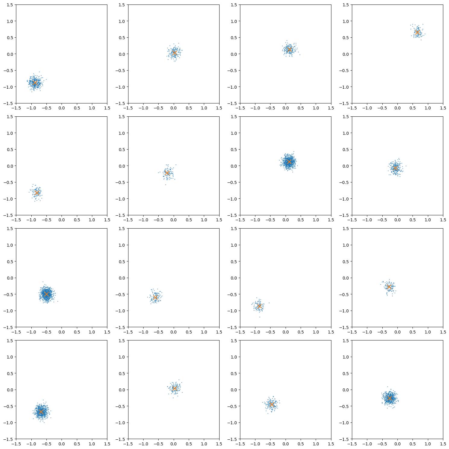
And then we’ll chuck the data and labels into a PyTorch dataloader.

from torch.utils.data import TensorDataset, DataLoader

dataset = TensorDataset(X, labels)
loader = DataLoader(dataset, batch_size=32, shuffle=True)

And then we train!

# ----------------
# 4. Training
# ----------------
from tqdm.notebook import trange
criterion = nn.BCEWithLogitsLoss()
optimizer = optim.Adam(model.parameters(), lr=0.005)
running_losses = []
# for epoch in range(100):
pbar = trange(100)
for epoch in pbar:
    running_loss = 0.0
    for X_batch, y_batch in loader:
        optimizer.zero_grad()
        theta, data = X_batch[:, 0].unsqueeze(1), X_batch[:, 1:]

        y_pred = model(theta, data)
        loss = criterion(y_pred, y_batch)
        loss.backward()
        optimizer.step()
        running_loss += loss.item() * X_batch.size(0)

    running_losses.append(running_loss/len(dataset))
    pbar.set_postfix({"Epoch": f"{epoch+1}", "Loss": f"{running_loss/len(dataset):.4f}"})

The subsequent loss curve, plus one more round of training with a lower learning rate looks like.

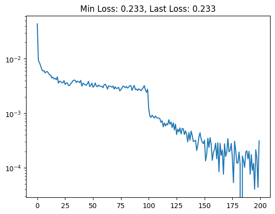
We can first check the accuracy of the classifier by giving it some new data and looking at the average prediction when we know the samples are correlated in the way we originally generated them, and when we know they aren’t.

with torch.no_grad():
    test_N = 10000000
    num_loglike = 20
    centres = generate_conditionals(n_samples=test_N)
    noise_multiplier= 1.
    sample = generate_data(centres, n_samples=1, noise_std = noise_multiplier*0.1).squeeze()

    prob = torch.sigmoid(model(sample, centres)).mean().item()

    print(f"Probability of being correlated (when correlated): {prob:.3f}")

    noise_multiplier= 10.
    sample = generate_data(centres, n_samples=1, noise_std = noise_multiplier*0.1).squeeze()

    prob = torch.sigmoid(model(sample, centres)).mean().item()

    print(f"Probability of being correlated (when not correlated): {prob:.3f}")

Probability of being correlated (when correlated): 0.861
Probability of being correlated (when not correlated): 0.164

Not bad, we don’t expect the classifier to get to 100%, in fact this would be a sign of pure overtraining.

Next we’ll look at example likelihood plots for random samples of the parameters and data.

with torch.no_grad():
    test_N = 1

    centres = generate_conditionals(n_samples=1)

    example_centres = torch.linspace(centres.squeeze()-1., centres.squeeze()+1., 501).unsqueeze(1)

    samples = generate_data(centres, n_samples=1).squeeze().repeat((len(example_centres), 1))


    print(samples.shape, example_centres.shape)
    loglike = model(samples, example_centres).squeeze()

    print(samples.shape, loglike.shape)

    plt.figure()
    plt.plot(example_centres.squeeze(), loglike.exp())
    plt.axvline(centres.squeeze(), c='tab:orange')
    plt.show()

One example plot looks like the below.

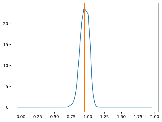
And then similar to my previous post for NPE and NLE, we can look at how often the true parameter value is within 1 std from the mode, 2 std and so on. It should match the relevant coverage for a standard normal distribution for the same number of sigma (e.g. the number of reconstructed values within 1 sigma should be ~68%)⁵.

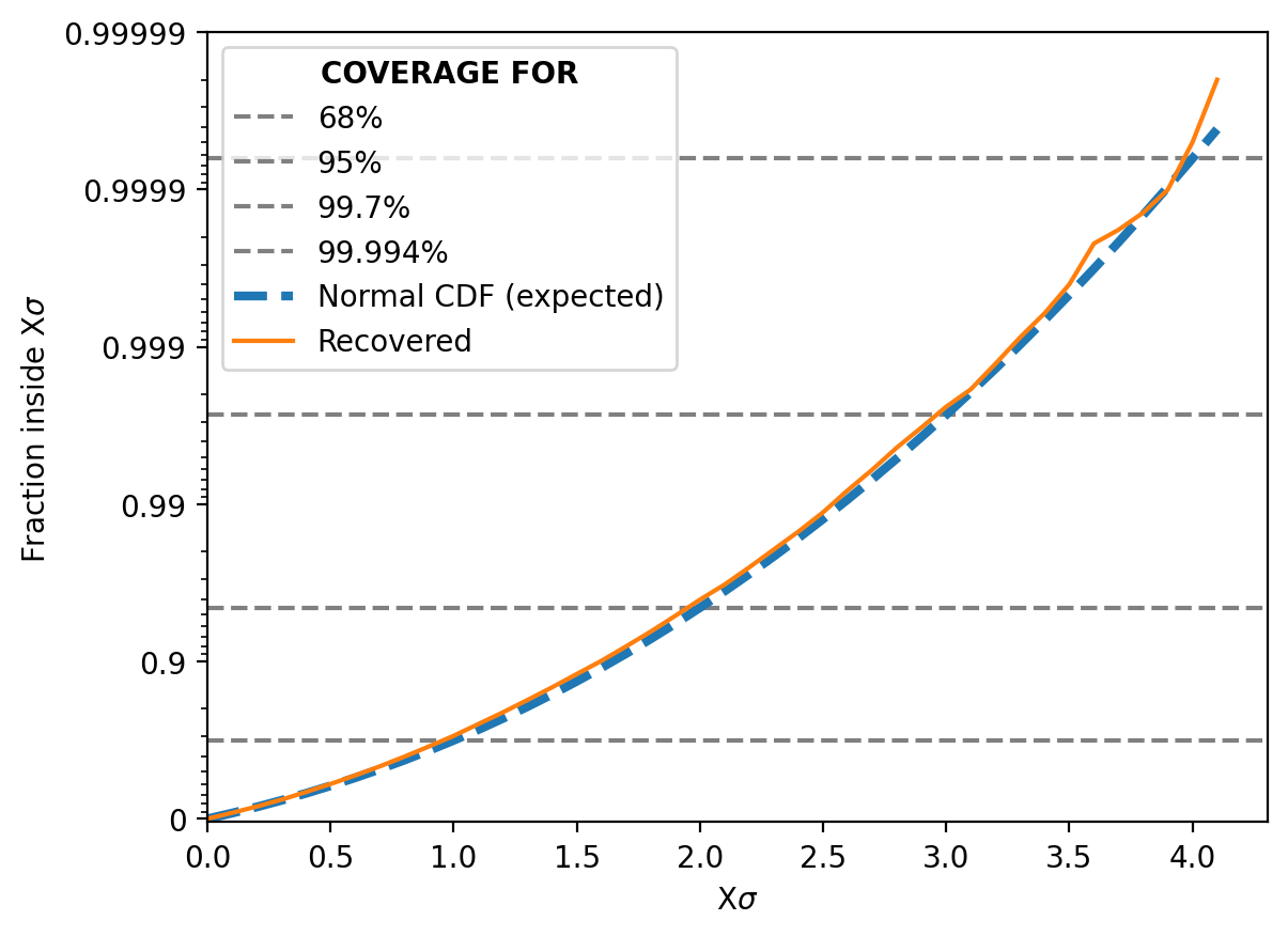
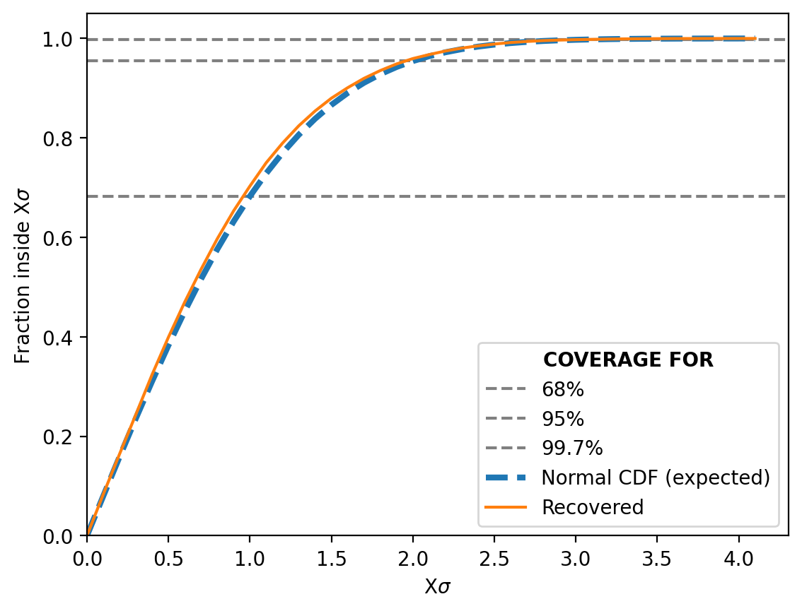
This shows that the NRE approximation of the likelihood is extremely good⁶ but not in an overtraining way. That would show up as deviations in the above, not the lines being almost identical.

Dataset Level Rudimentary Implementation

Beyond creating a likelihood representation on a per observation level we can additionally look at the likelihood for a given dataset. The math works out exactly the same except that the concept of “datapoint” for \(\vec{x}\) is broadened to “data”. We then create the labels in the same way looking for when conditional-/hyper-parameters are related to data/datasets.

The key difficulty is that we can’t just chuck the data into the neural network anymore and we need to aggregate the data within a given dataset. Again similar to my previous posts, an easy way that we can do this is with an embedding network. In which we feed in the data and get some compressed representation that we can use to feed into our classifier. I will use a Deep Set neural networks to achieve this rather than simple summary statistics.

The paper on Deep Set neural networks I’ve used as reference above gets a little in the weeds for the purpose of this post. The setup can simply be denoted as three functions: \(\{\vec{y}_i\}_i\)⁷ inputs for \(i\in \{1,..., S\}\), a single neural network that acts on each data point individually \(\phi\), some sort of aggregation function/statistics \(f\) such as the mean, and a second neural network that takes the output of the aggregated data \(\Phi\).

Putting this into some code.

import torch
import torch.nn as nn
import torch.nn.functional as F

class DeepSet(nn.Module):
    def __init__(self, input_dim, output_dim, phi_hidden=32, Phi_hidden=32):
        super().__init__()
        
        self.phi = nn.Sequential(
            nn.Linear(input_dim, phi_hidden),
            nn.ReLU(),
            nn.Linear(phi_hidden, phi_hidden),
            nn.ReLU(),
            nn.Linear(phi_hidden, phi_hidden),
            nn.ReLU(),
        )
        
        self.Phi = nn.Sequential(
            nn.Linear(phi_hidden, Phi_hidden),
            nn.ReLU(),
            nn.Linear(Phi_hidden, Phi_hidden),
            nn.ReLU(),
            nn.Linear(Phi_hidden, output_dim),
        )


    def forward(self, x):
        """
        x: [batch_size, set_size, input_dim]
        """
        phi_x = self.phi(x)  # [batch_size, set_size, phi_hidden]
        
        # Aggregate along the data dimension which we'll say is 1
        agg = phi_x.mean(dim=1)

        # Apply Phi to aggregated vector
        out = self.Phi(agg)

        return out

This allows us to create a fixed size output, or embedding, for use in our analysis, and later on can be slightly adjusted to deal with changes in dataset size as part of the training.

This means that our code stays almost exactly the same except we first feed the data into this embedding network and then into the neural network. Here it is with the slight changes though.

class NRE(nn.Module):
    def __init__(self, data_dim=1, theta_dim=1, embedding_size=2, hidden_nodes=16):
        super().__init__()

        self.embedding_net = DeepSet(input_dim=data_dim, output_dim=embedding_size, phi_hidden=hidden_nodes, Phi_hidden=hidden_nodes)


        combined_dims = theta_dim + embedding_size

        # Binary net does not change a lick
        self.binary_net = BinaryNet(combined_dims, hidden_nodes=hidden_nodes)


    def forward(self, data, theta):
        # assuming that the input shapes are (batch_dim, data/theta dim)
        embedding_output = self.embedding_net(data)

        combined_dataset = torch.concat((embedding_output, theta), dim=1)

        return self.binary_net(combined_dataset)

model = NRE(data_dim=2, theta_dim=1, embedding_size=5)

So we have the same data and parameter dimensionality but we’ve set the dimensionality of the embedding to 5⁸.

Now let’s test it out, we’ll use the same setup, just generate multiple datapoints for each value of the hyperparameter.

N_data_samples = 100

theta_base = generate_conditionals(n_samples=N_hyp_samples)

y_noisy = generate_data(theta_base, n_samples=N_data_samples).squeeze()

We’ll then set up our data a little differently to before due to the shape change in y_noisy, but the broad aspects remain the same. We generate permutation of their indices and apply them to all the relevant tensors.

# Generate labels for whether the samples are
pos_labels = torch.ones((N_hyp_samples, 1))
    # or are not related
neg_labels = torch.zeros((N_hyp_samples, 1))
# and then combine them into a single tensor
labels = torch.vstack([pos_labels, neg_labels])

# Generating the random index slices
shuffled_indices = torch.randperm(N_hyp_samples)

# Combining the joint dist samples together
pos_hyp_samples = torch.vstack([theta_base, theta_base])
# And making the marginal dist samples by shuffling the data values
pos_data_samples = torch.vstack([y_noisy, y_noisy[shuffled_indices]])

# Then creating one more layer of permutations so the classifier
    # doesn't just learn the ordering
perm = torch.randperm(len(labels))

pos_hyp_samples = pos_hyp_samples[perm]
pos_data_samples = pos_data_samples[perm]
labels = labels[perm]

Loading this into some PyTorch dataloaders…

from torch.utils.data import TensorDataset, DataLoader

dataset = TensorDataset(pos_hyp_samples, pos_data_samples, labels)
loader = DataLoader(dataset, batch_size=64, shuffle=True)

And then training the classifier…

from tqdm.notebook import trange
criterion = nn.BCEWithLogitsLoss()
optimizer = optim.Adam(model.parameters(), lr=0.005)
running_losses = []

pbar = trange(100)
for epoch in pbar:
    running_loss = 0.0
    for theta_batch, data_batch, y_batch in loader:
        optimizer.zero_grad()

        y_pred = model(data_batch, theta_batch)
        
        loss = criterion(y_pred, y_batch)
        loss.backward()
        optimizer.step()
        running_loss += loss.item() * theta_batch.size(0)

    running_losses.append(running_loss/len(dataset))
    pbar.set_postfix({"Epoch": f"{epoch+1}", "Loss": f"{running_loss/len(dataset):.4f}"})

And then similar to above we get that for actually correlated samples we have a 98% chance of them being correlated and then for not correlated samples (at least in the way we generated them) a probability of correlation of 13%. So our classifier is doing relatively well as a classifier.

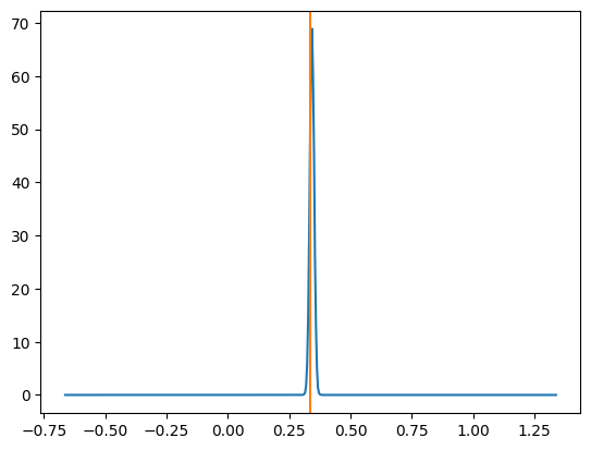
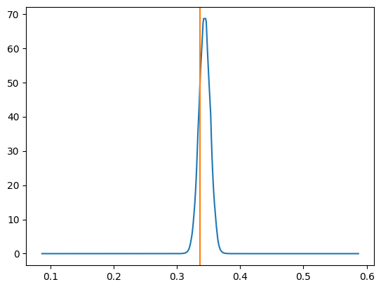
Now let’s look at what our approximated log-likelihood ratio curves look like. You can observe that the width of the distribution is smaller than the above example which makes sense as we’re using more data (hence the zoomed in right plot).

We can then also look at the Simulation-Based Calibration test or the “coverage” (not a commonly used term) as I explained it above.

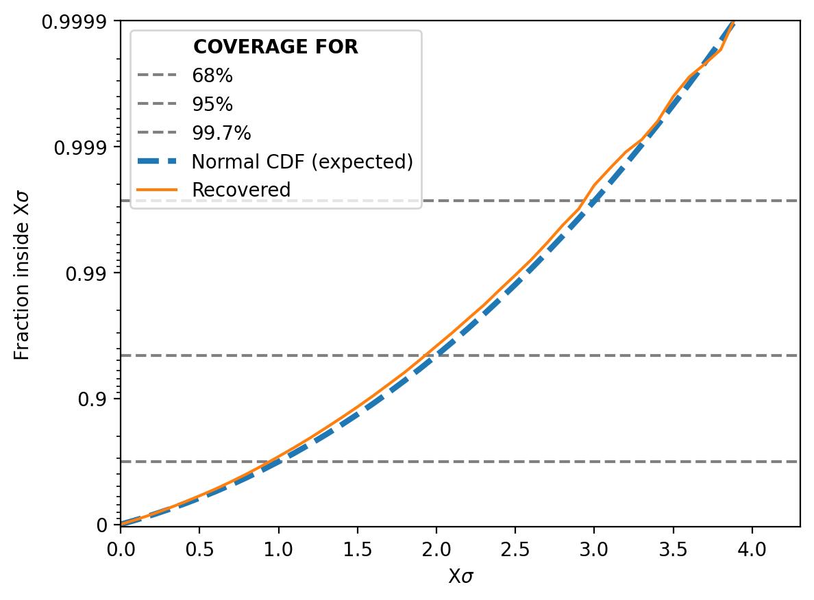
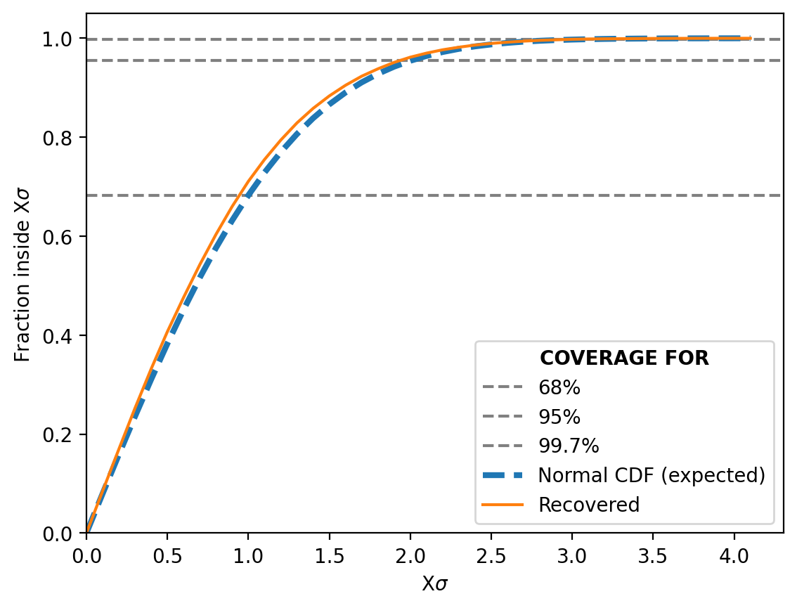
And it does just as well if not even better than before!

Conclusion

My honest response to this when I first saw it was….

There are many benefits to this approach, mostly coming from it being SBI (e.g. not having to directly model nuisance parameters) and the ability to now have a likelihood with in-built gradients, but there are a few caveats to using it:

1. This is a likelihood estimation technique, if you want a posterior you will typically need to run the result through another round of analysis.
2. Overtraining the classifier equates to not having a representative likelihood. If your data is from simulations there is always chance that the classifier will only work on those and not on real data. To check if this could be the case would require more testing and a longer post that I don’t want to subject you to at the moment.
3. You are training a likelihood ratio and not a likelihood, meaning that combining datasets through basic multiplication is not immediately justifiable in the strictest sense.

But it is amazing that something so simple can enable us to possibly expand our analysis greatly through not having to directly model nuisance parameters, to amortising our inference (re-running the analysis is just a forward pass through a neural network) and get a cheap representation of a dataset or observation level likelihood.