In this post, I’ll attempt to give an introduction to simulation-based inference specifically delving into the methods NPE and NLE including rudimentary implementations.

Resources

As usual, here are some of the resources I’m using as references for this post. Feel free to explore them directly if you want more information or if my explanations don’t quite click for you.

• A robust neural determination of the source-count distribution of the Fermi-LAT sky at high latitudes by Eckner et al.
• The frontier of simulation-based inference by Kyle Cranmer, Johann Brehmer and Gilles Louppe
• Recent Advances in Simulation-based Inference for Gravitational Wave Data Analysis by Bo Liang and He Wang
  • Really recommend giving this a read, it’s hard to find papers that discuss the general topics without getting into the weeds of the specific implementation that they are trying to advocate for or simply too vague.
• Consistency Models for Scalable and Fast Simulation-Based Inference
• Missing data in amortized simulation-based neural posterior estimation
  • Only paper I’ve read that directly and nicely talks about using aggregator networks for variable dataset sizes

Table of Contents

• Motivation
• Core Idea
• Neural Posterior Estimation (NPE)
  • Can I trust this?
• Neural Likelihood Estimation (NLE)
• Conclusion

Motivation

The TLDR of simulation-based-inference (SBI)¹ is that you have a prior on some parameters \(\vec{\theta}\) and a simulator \(g\), which can give you realistic data \(\vec{x}=g(\vec{\theta})\), you then utilise advances in machine learning to learn the likelihood or posterior from this without having to actually specify the likelihood directly^{1 2}.

The benefits of SBI include but are not limited to:

1. The ability to handle large numbers of nuisance parameters (see above)
2. The user does not have to specify the likelihood allowing direct inference if a realistic simulator already exists (e.g. climate modelling) even if the strict likelihood would be intractable.
3. There have been a few works showing that SBI methods can better handle highly non-gaussian and highly-multi-modal relationships within probability distributions
4. Amortised inference, you can train a model to approximate the probabilities for a dataset and then re-use them for other observations relatively trivially
5. Through the use of the simulators and neural networks involved, SBI is generally easier to parallelise
6. Efficient exploration of parameter space, through the fact that the simulator will often only output realistic data (by design), the algorithms don’t have to waste time in regions of the parameter space that don’t lead to realistic data.

The ability to handle a large number of nuisance parameters is actually what sparked my interest in SBI through the paper A robust neural determination of the source-count distribution of the Fermi-LAT sky at high latitudes by Eckner et al. who used Nested Ratio Estimation (a variant of NRE, which I’ll discuss in my next post) to analyse data with a huge number of nuisance parameters introduced by an unknown source distribution in the gamma-ray sky.

I would recommend looking at The frontier of simulation-based inference by Kyle Cranmer, Johann Brehmer and Gilles Louppe and the references therein to check these claims out for yourself if you want.

And more recently, I came across this great paper by Bo Liang and He Wang called Recent Advances in Simulation-based Inference for Gravitational Wave Data Analysis that discusses the use of SBI within gravitational wave data analysis (in the title I know) but it also discusses some of the popular SBI methods in use as of writing. So, I thought I would try and touch on how each of them work in a little more detail than the paper allowed and try to make it a little more general, additionally showing some rudimentary implementations of some of them, with the end goal really being understanding everything in the below figure (Fig. 1 from the paper).

In this post I will go through Neural Posterior Estimation and Neural Likelihood Estimation and in later posts Neural Ratio Estimation, Classifer-based Mutual Posterior Estimation and finally Flow Matching Posterior Estimation (rough order of how hard it will be to make rudimentary implementations).

Core Idea

First we assume that one has priors for the set of hyperparameters that theoretically influence the data of a given system. e.g.

where \(\vec{\theta}\) is the set of hyperparameters we are interested in. And further assume (for now) that either:

• the set of nuisance parameters \(\vec{\eta}\) can be further sampled based on these values,
• or that the two sets are independent.

Taking the stronger assumption of independence as it is often not restricting in practice,

Denoting the simulator that takes in these values and outputs possible realisations of the data as \(g\) then,

This is in effect samples from the likelihood and with this we have samples from the joint probability distribution through Bayes’ theorem with marginalisation over the nuisance parameters ,

This assumes that we can robustly sample over the space of nuisance parameters. We can simultaneously marginalising them out³ when generating the samples such that⁴,

Now because we have these samples, we can try and approximate the various densities that are behind them, using variational approximations such as normalising flows, variational autoencoders, binary classifiers etc. And that’s SBI, the different methods differ in specifically how they choose to model these densities (e.g. flow vs VAE vs classifier vs etc) and importantly which densities they are actually trying to approximate. e.g. Neural Posterior Estimation directly models the posterior density \(p(\vec{\theta}\vert\vec{x})\), while Neural Likelihood Estimation tries to model the likelihood \(\mathcal{L}(\vec{x}\vert \vec{\theta})\). We’ll start with Neural Posterior Estimation or NPE.

Neural Posterior Estimation (NPE)

Continuing off from where we left the math, we can then try and estimate the density \(p(\vec{\theta}\vert\vec{x})\), more simply known as the posterior, with some variational approximation \(q(\vec{\theta}\vert \vec{x})\) such as conditional normalising flows through the forward KL divergence.

We train the variational approximation to the distribution by optimising over the parameters that dictate the shape of said approximation, \(\vec{\varphi}\), that are separate to the parameters of the actual problem we are trying to solve. Meaning, that our KL divergence looks more like,

where I use the symbol “\(;\)” to specifically highlight the dependence through the variational approximation and not the conditional dependencies in the density that we are trying to model⁵.

During training, all that we trying to do is minimise this divergence with respect to the parameters \(\vec{\varphi}\). Hence from this perspective, the first term inside the divergence is a constant, and plays no part in the loss function we are trying to optimise. So the final form of the loss that we are trying to minimise is⁶,

This is no different to what I went through in my post on conditional normalising flows, however, the thing that then makes this super-useful for variational inference is that \(\vec{x}\) doesn’t have to represent a single observation, but can be a whole dataset.

The dependency works in the exact same way, just that instead of a vector \(\vec{x}\) is more of a matrix, and we average over the dimension corresponding to different realisations of the hyper-parameters.

In essence:

• If I have a set of hyper-parameters, \(\vec{\theta}_i\),
• then produce a dataset \(\vec{x}_{i,j}\)
  • the \(i\) subscript denotes which hyper-parameter the datapoint came from
  • the \(j\) denotes the \(j^\text{th}\) datapoint for the given hyper-parameter.
  • Emphasizing that it is still a “vector”, it does not have to be a single value, but I refuse to use tensors in a general audience post even though that’s basically what I’m using
• we aggregate over/learn a simpler representation for \(j\) and the data dimension (I’ll touch on this in a second)
• we then average over \(i\)

The complication is that this would be dependent on the size of the datasets that we produce in our simulations during training. If I use 10,000 samples in my training, my posterior representation would only be suitable for \(\sim\) 10,000 samples, not for \(\lesssim\) 9,000 or \(\gtrsim\) 11,000. But I just told you that all this is great at amortised inference where you don’t have to redo training for new data?! What gives? Well unfortunately standard NPE as far as I know only deals with fixed input sizes. It is still great at amortised inference when you want to re-run the analysis on datasets of the same size.

In a later post I hope to show how you can train for dataset size using Deep Set neural networks and summary statistics. But the fact still remains that we want our setup to be re-useable for different dataset sizes. We don’t want to have to rework the whole setup for a different number of observations. For that I will use Deep Set neural networks, partly as a primer for when I touch on training with differently sized datasets.

The paper on Deep Set neural networks I’ve used as reference above gets a little in the weeds for the purpose of this post. The setup can simply be denoted as three functions: \(\{\vec{y}_i\}_i\)⁷ inputs for \(i\in \{1,..., S\}\), a single neural network that acts on each data point individually \(\phi\), some sort of aggregation function/statistics \(f\) such as the mean, and a second neural network that takes the output of the aggregated data \(\Phi\).

Putting this into some code.

import torch
import torch.nn as nn
import torch.nn.functional as F

class DeepSet(nn.Module):
    def __init__(self, input_dim, output_dim, phi_hidden=32, Phi_hidden=32):
        super().__init__()
        
        self.phi = nn.Sequential(
            nn.Linear(input_dim, phi_hidden),
            nn.ReLU(),
            nn.Linear(phi_hidden, phi_hidden),
            nn.ReLU(),
            nn.Linear(phi_hidden, phi_hidden),
            nn.ReLU(),
        )
        
        self.Phi = nn.Sequential(
            nn.Linear(phi_hidden, Phi_hidden),
            nn.ReLU(),
            nn.Linear(Phi_hidden, Phi_hidden),
            nn.ReLU(),
            nn.Linear(Phi_hidden, output_dim),
        )


    def forward(self, x):
        """
        x: [batch_size, set_size, input_dim]
        """
        phi_x = self.phi(x)  # [batch_size, set_size, phi_hidden]
        
        # Aggregate
        agg = phi_x.mean(dim=1)

        # Apply Phi to aggregated vector
        out = self.Phi(agg)

        return out

This allows us to create a fixed size output, or embedding, for use in our analysis, and later on can be slightly adjusted to deal with changes in dataset size as part of the training.

To test how this works we’ll first generate some data to work with using the make_moons function from the scikit-learn package where we have

• a mixture parameter \(d\) for what fraction of samples come from the upper moon of the double moon distribution
• a gaussian noise parameter \(\sigma_c\)
• a vertical dilation factor \(t_{\text{dil}}\)

# training samples
n_hyp_samples = 10000
n_data_samples = 200 # constant dataset sizes for now

training_conditional_samples = sample_conditionals(n_samples=n_hyp_samples).T
training_n_samples = n_data_samples*torch.ones((n_hyp_samples),)
_training_data_samples = []
for train_n_sample, cond_samples in zip(training_n_samples, training_conditional_samples):
    # print(train_n_sample.dim())
    _training_data_samples.append(ln_like.rsample(cond_samples, n_samples=train_n_sample))


training_data_samples = np.array(_training_data_samples)
training_data_samples = torch.tensor(training_data_samples).transpose(1, 0).squeeze()

Now we use the exact same RealNVP setup I had in my previous post except for the initialisation which now uses the DeepSet neural network.

class RealNVPFlow(nn.Module):
    def __init__(self, num_dim, num_flow_layers, hidden_size, cond_dim, embedding_size):
        super(RealNVPFlow, self).__init__()

        self.dim = num_dim
        self.num_flow_layers = num_flow_layers

        self.embedding_size = embedding_size

        ################################################
        ################################################ 
        # setup base distribution
        self.distribution = dist.MultivariateNormal(torch.zeros(self.dim), torch.eye(self.dim))


        ################################################
        ################################################ 
        # setup conditional variable embedding


        self.cond_net = DeepSet(input_dim=cond_dim, output_dim=embedding_size, phi_hidden=hidden_size, Phi_hidden=hidden_size)
        # *[continues after this but there are no changes]*

And the training loop will be a little different as the size of the data samples will be different to the size of the hyperparameter samples. I could add a new axis to them and repeat along it but that would be wasted memory, so the training loop now has two data loaders: one for hyperparameter samples and one for the data samples. Looking like the following.

import tqdm
import numpy as np
from copy import deepcopy
from torch.utils.data import TensorDataset, DataLoader


def train(model, hyp_param_samples, data_samples, epochs = 100, batch_size = 128, lr=1e-3, prev_loss = None):
    # print(data.shape)
    train_hyper_loader = torch.utils.data.DataLoader(hyp_param_samples, batch_size=batch_size)
    train_data_loader = torch.utils.data.DataLoader(data_samples, batch_size=batch_size)
    optimizer = torch.optim.Adam(model.parameters(), lr=lr)
    
    if prev_loss is None:
        losses = []
    else:
        losses = deepcopy(prev_loss)

    with tqdm.tqdm(range(epochs), unit=' Epoch') as tqdm_bar:
        epoch_loss = 0
        for epoch in tqdm_bar:
            for batch_index, (training_hyper_batch, training_data_batch) in enumerate(zip(train_hyper_loader, train_data_loader)):

                log_prob = model.log_probability(training_hyper_batch, training_data_batch)
                    
                # print("final log_prob.shape: ", log_prob.shape)
                loss = - log_prob.mean(0)

                # Neural network backpropagation stuff
                optimizer.zero_grad()
                loss.backward()
                optimizer.step()

                epoch_loss += loss
            epoch_loss /= len(train_hyper_loader)
            losses.append(np.copy(epoch_loss.detach().numpy()))
            tqdm_bar.set_postfix(loss=epoch_loss.detach().numpy())

    return model, losses

And all that’s left is to chuck everything into our model and train.

torch.manual_seed(2)
np.random.seed(0)

num_flow_layers = 8
hidden_size = 16


NVP_model = RealNVPFlow(num_dim=3, num_flow_layers=num_flow_layers, hidden_size=hidden_size, cond_dim=2, embedding_size=4)
trained_nvp_model, loss = train(NVP_model, hyp_param_samples=training_conditional_samples, data_samples=training_data_samples, epochs = 500, lr=1e-3, batch_size=1024)

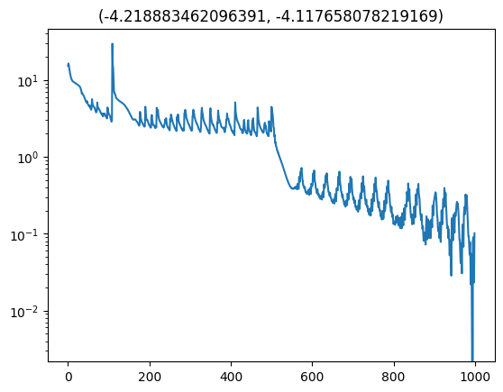
With a couple extra things regarding the training (which if included would just make the point of this point more cloudy… cloudier?) we arrive at the following loss curve. Excuse the lack of labels, the x-axis is iterations and the y is the translated loss so that the minimum is at 0.

Now we have an approximate conditional distribution for our posterior! Meaning that we can give it different realisations of the data and the time it takes to go through the neural networks is the time it takes to get posterior samples (i.e. amortised inference). Let’s have a look at a few of these.

And another.

And another because why not.

You might be wondering why the second two don’t seem to do so well in regards to recovering the true value. Well actually I chose this exactly because they don’t, because we are modelling a probability distribution if we recover the true values 100% within the \(1\sigma\) contour then we are not modelling a probability distribution as the true values should like within \(1\sigma\) roughly 68% of the time, otherwise it’s not a probability distribution. This actually leads into the next subsection.

Can I trust this?

The question that should have been and currently is at the back of your mind is “Can I actually trust this?” And the answer to that is not straightforward.

The two questions inside “Can I trust this?” that I am asking myself are:

1. Is the simulated data a realistic representation of the actual data?
   • I can’t do that well for this post seeing as I don’t have real data however, I’d recommend this paper which touches on it.
2. Have I adequately covered my space of hyperparameters during training?
   • So that my eventual data that I analysis comes from an area of the parameter space that I have adequately trained on

The second one we can partly tackle here. One way we can test this is through a standard Simulation-Based Calibration test. This is basically checking that if you have a known set of true hyperparameters and you simulate data from them, that the analysis setup/posterior recover these true values within \(1\sigma\) 68% of the time, within \(2\sigma\) 95% of the time and so on.

Seeing as generating data and analysing it is really quick, because of the very nature of what we are trying to do with amortised inference, we can just:

1. randomly sample our prior,
2. generate data,
3. run this data through our conditional density estimator,
4. store how far the true value for the hyperparameter is to the recovered mean of the relevant samples
5. create a simple distribution for what fraction of runs had the true value within \(1\sigma\), \(1.1\sigma\) and \(2\sigma\) and so on comparing it to the expected values⁸

We’ll run this for 2000 iterations and plot the result in steps of \(0.1\sigma\).

Woo! Our probability distribution is being a good probability distribution (purely as far as probabilities go, not necessarily accuracy to the system per say). The one slight hiccup is that it seems our pipeline is over-estimating the width of the distribution for large sigma values. This is likely one an artefact of actually not covering the parameter space during training as mentioned above.

More modern/better implemented methods of NPE, e.g. SNPE, actually focus in on difficult areas of the parameter space during training to (in part) try and solve this. This however, introduces a potential bias in the now adjusted hyper-parameter proposal function \(\tilde{p}(\vec{\theta})\) which is not necessarily equal to \(\pi(\vec{\theta})\) (our prior) as we are now learning \(p_0(\vec{\theta}\vert\vec{x})=\mathcal{L}(\vec{x}\vert\vec{\theta}) \tilde{p}(\vec{\theta})/C_0\) instead of \(p(\vec{\theta}\vert\vec{x})=\mathcal{L}(\vec{x}\vert\vec{\theta}) \pi(\vec{\theta})/C\)

This kind of bias has a much more minimised effect for neural likelihood estimation.

Neural Likelihood Estimation

In neural likelihood estimation or NLE, we instead try to approximate the likelihood for data instead of the posterior. This avoids the bias in the prior proposal as it isn’t directly involved in the quantity we are trying to find. I will focus on training it for a single datapoint as we couldn’t really do that for NPE, but know that you could do a very similar thing as we did above for whole datasets. There are two caveats to taking this route though:

1. If you want the probability of your parameters given the data, the posterior \(p(\vec{\theta}\vert\vec{x})\), then we need to further run the analysis again using something like MCMC for example. We essentially get a cheap and variable version of the likelhood where
   • however in this new likelihood we potentially don’t have to care about some unknown nuisance parameters anymore
   • and we get a likelihood that we can pass gradients through to use HMC
2. Now our data has to be continuous if we want to use something like a normalising flow to approximate them (although this is not true for Neural Ratio Estimation)
   • but now our hyperparameters don’t have to be continuous

This setup more closely follows that of my previous post on conditional normalising flows as the number of conditional variables is now smaller than the number of density variables.

So now our data is still the moon distributions, and our parameters will be the same except we’ll use our new ability of discrete parameters to look at whether our data came from the upper (=1) or lower moons (=0) re-using our variable name \(d\). With the same simulator…

We’ll make our prior give us samples that follow:

And using the same conditional embedding network as the post.

import torch
import torch.nn as nn

class ConditionEmbedding(nn.Module):
    def __init__(self, input_dim=2, embedding_size=4, embed_hidden_dim=64):
        super().__init__()
        self.point_net = nn.Sequential(
            nn.Linear(input_dim, embed_hidden_dim), nn.ReLU(),
            nn.Linear(embed_hidden_dim, embed_hidden_dim), nn.ReLU(),
            nn.Linear(embed_hidden_dim, embedding_size), nn.ReLU())

    def forward(self, x):

        per_point = self.point_net(x)
        return per_point

Changing our RealNVP class to use this instead.

class RealNVPFlow(nn.Module):
    def __init__(self, num_dim, num_flow_layers, hidden_size, cond_dim, embedding_size):
        super(RealNVPFlow, self).__init__()

        self.dim = num_dim
        self.num_flow_layers = num_flow_layers

        self.embedding_size = embedding_size

        ################################################
        ################################################ 
        # setup base distribution
        self.distribution = dist.MultivariateNormal(torch.zeros(self.dim), torch.eye(self.dim))


        ################################################
        ################################################ 
        # setup conditional variable embedding


        self.cond_net = ConditionEmbedding(input_dim=cond_dim, embedding_size=embedding_size, embed_hidden_dim=hidden_size)

With the training objective being the same as the previous section except we switch the dependencies in the density we are trying to fit.

And to keep this short, and seeing as I’m literally running the exact same code as in the post, I’ll refer you to my previous post for training. But let’s presume now that we’ve fit the density, and hence can generate datasets based on the conditional variables/our hyper-parameters.

Where I generated the above by generating the conditional parameters.

_training_conditional_samples = sample_conditionals(n_samples=1).squeeze()

Generated data samples using our approximated likelihood.

samples = trained_nvp_model.rsample(5000, _training_conditional_samples)

And then we can directly look at the probability values for the samples.

trained_nvp_model.log_probability(
    torch.tensor(samples), 
    torch.tensor(_training_conditional_samples)
    ).sum()

And now that we have this we can throw it into an MCMC or nested sampler for example to get our posterior. I would not recommend doing it this way but it does the job.

from dynesty import NestedSampler

# Sample true values
_posterior_gen_conditional_samples = sample_conditionals(n_samples=1).squeeze()

# Get data from true values
_posterior_gen_data_samples = cond_ln_like.rsample(_posterior_gen_conditional_samples, n_samples=500)

with torch.no_grad():

    
    def prior_transform(u):
        d_samples = _d_conditional_dist.sample((1,)).squeeze()
        log10_sigma_samples = _noise_conditional_dist.sample((1,)).squeeze()
        t_shift_samples = _t_shift_conditional_dist.sample((1,)).squeeze()

        output = np.array([d_samples, log10_sigma_samples, t_shift_samples])

        return output


    def ln_like(x):

        # matching shapes with how conditional density was trained
            # gives it a shape of (500, 3)
        torched_x = torch.tensor(x).repeat((500, 1))
        
        ln_like_val = trained_nvp_model.log_probability(_posterior_gen_data_samples, torched_x)

        ln_like_val = torch.where(torch.isnan(ln_like_val), -torch.inf, ln_like_val)

        return float(ln_like_val.sum())

    sampler = NestedSampler(prior_transform=prior_transform, loglikelihood=ln_like, ndim=3, nlive=300)

    sampler.run_nested(dlogz=0.5, print_progress=True)

    sampler_results = sampler.results()

    ns_sampler_samples = sampler_results.samples_equal()

Which gave me the following approximate corner density plot (remember the \(d\) is discrete on 0 or 1).

I will say thought that I had to increase the number of training samples of the NLE density to get this to work which brings me to the conclusion.

Conclusion

These methods are really interesting but do have a few caveats. Mostly because of the way that I implemented them.

1. The methods both rely on that you’ve sampled the space of hyper-parameters well enough that they are accurate in the area of interest on real datasets.
2. The simulators have to realistically represent the data.
3. Your approximation method is expressive enough to properly represent the given distribution. (e.g. the flow has to be expressive enough to actually represent the exact one well enough)

The first is mostly solved be sequential methods that localise the training in difficult areas of the hyper-parameter space. And the second is dependent on the given system.

Additionally, there is a trade off between initial training. The idea of amortised inference is that there is a large initial cost, reducing the overall by reduced computation time for following analyses.

In the following post I’ll tackle the next method mentioned above, Nested Ratio Estimation, which relies on a binary classifier to approximate the likelihood.