
Building a normalising flow from scratch using PyTorch
Published:
In this post I will attempt to show you how to construct a simple normalising flow using base elements from PyTorch heavily inspired by a similar post by Eric Jang doing the same thing with TensorFlow from 2018 and subsequently his tutorial using JAX from 2019.
Resources
I’m just going to say to head over to Eric Jang’s tutorial again + a paper with extremely clear math for how this post works + a demonstrative RealNVP paper.
- Normalizing Flows Tutorial, Part 1: Distributions and Determinants
- Normalizing Flows Tutorial, Part 2: Modern Normalizing Flows
- Normalizing Flows in 100 Lines of JAX
- Normalizing Flows for Probabilistic Modeling and Inference
- Which I’ll refer to as Papamakarios linking directly to the pdf
- Density Estimation Using Real NVP
Table of Contents
- Background
- RealNVP Flow Class
- RealNVP Transformation Layer Class
- Approximating a sample distribution with normalising flows
- Approximating an unknown unnormalised distribution
- Conclusion
Background
In today’s post we will try and do two things: 1. approximate a sample distribution using normalising flows (easy), and 2. approximating an unknown unnormalised probability distribution (not as easy but not hard?) specifically with a RealNVP style normalising flow.
I’m going to mostly assume (probably wrongly) that you have already looked through my original normalising flows post, but the TLDR of it is that we have a way to produce analytical probability distributions by stacking a bunch of simple transformations on top of a simple analytical base distribution that allows you to model pretty complex behaviour. Like so,
\[\begin{align} p_\mathbf{x}(\mathbf{x}) &= p_\mathbf{u}(\mathbf{u}) \vert J_T(\mathbf{u})\vert^{-1} \\ &= p_\mathbf{u}(T^{-1}(\mathbf{x})) \vert J_{T^{-1}}(\mathbf{x}) \vert\\ \end{align}\]where \(\mathbf{u} = T^{-1}(\mathbf{x})\) (equations 2 and 3 in Papamakarios). \(J_T\) is the Jacobian for the transformations \(T\),
\[\begin{align} J_T(\mathbf{u}) = \left[ \begin{matrix} \frac{\partial T_1}{\partial u_1} & \ldots & \frac{\partial T_1}{\partial u_D} \\ \vdots & \ddots & \vdots\\ \frac{\partial T_D}{\partial u_1} & \ldots & \frac{\partial T_D}{\partial u_D}\\ \end{matrix} \right]. \end{align}\](Equation 4 in Papamakarios). And if we stack these transformations, that are assumed to be bijective, then it’s handy to know that the inverse of their composition is the composition of their inverses (in reverse order) and that the determinant jacobian of the subsequent total transformation is the product of their individual determinants (equations 5 and 6 in Papamakarios). The usual goal of different normalising flows is to balance expressivity and the complexity of calculating the transformations’ inverses and determinants.
The general process is shown in Fig. 2 of Papamakarios

As an example of the power of this method I showed in the addendum of my original post that you could model large and complex posteriors like the one below.
")
However, for this I relied on inbuilt classes and methods within the Python package Pyro to do the actual modelling. In this post we’re going to throw that away and also look at how we can approximate sample distributions with flows building everything from ‘scratch’ meaning using the inbuilt methods in PyTorch.
RealNVP Flow Class
A widely successful and relatively simple iteration of normalising flows is the RealNVP model that uses what we call a blocked coupling function for it’s transformations.
‘Block’ refers to a kind of transformation where if the parameter space that you are trying to model is \(D\)-dimensional, then we pick some integer \(d<D\) (typically just roughly half of \(D\)) such that the transformation \(T\) for input \(x\) and output \(y\) can be expressed as,
\[\begin{align} y_{1:d} &= x_{1:d} \\ y_{d+1:D} &= f(x_{d+1:D} \, \vert \, x_{1:d} ). \end{align}\]The notation \(1:d\) and \(d+1:D\) imitates the kind of slicing behaviour you’re likely familiar with in coding, referring to indices \(1\) to \(d\) and \(d+1\) to \(D\). Hence, the jacobian of the transformation follows,
\[\begin{align} J_T = \frac{\partial y}{\partial x} &= \left[ \begin{matrix} \mathbb{I}_d & \vec{\mathbf{0}} \\ \frac{\partial y_{d+1:D}}{\partial x_{1:d}} & \frac{\partial f}{\partial x_{d+1:D}}(x_{d+1:D} \vert x_{1:d})\\ \end{matrix} \right]. \end{align}\](The arrow on the \(\vec{\mathbf{0}}\) is to emphasize that this is a matrix). The beauty of this is that due to the block nature of the transformation, we can make the dependency of \(f\) on \(x_{1:d}\) as complicated and convoluted as we like (almost). As, the derivatives will be calculated automatically (if we implement it in TensorFlow, PyTorch or JAX) and the jacobian will just be the determinant of \(\frac{df}{\partial x_{d+1:D}}(x_{d+1:D} \vert x_{1:d})\) where the complicated dependencies are not a part of the derivative!
In the case of RealNVP the function \(f\) is affine described via the following,
\[\begin{align} y_{1:d} &= x_{1:d} \\ y_{d+1:D} &= x_{d+1:D} \odot \exp(s(x_{1:d})) + t(x_{1:d}). \end{align}\](the \(\odot\) refers to element-wise multiplication) The transformation seems like it only applies a simple dilation and shift, which is what it does, but it allows very non-linear behaviour through the fact that these shifts and dilations have a dependence on the other blocks of variables. The jacobian is then,
\[\begin{align} J_T &= \left[ \begin{matrix} \mathbb{I}_d & \vec{\mathbf{0}} \\ \frac{\partial y_{d+1:D}}{\partial x_{1:d}} & \textrm{diag} \left(\exp\left[ s(x_{1:d}) \right] \right)\\ \end{matrix} \right]. \end{align}\]Again, although we can have extremely complicated and non-linear behaviour through the dependence of the functions \(s\) and \(t\), the actual value of the jacobian’s determinant will be a simple product of the output of the function \(\exp\left(\left[ s(x_{1:d}) \right]\right)\)1.
In addition, the above allows us to sample our flow by generating said samples in the space of our simple distribution (in the above this would be adjacent to the values of \(x\)) but we also want to evaluate the probability of our model at different points in our parameter space. Meaning that we need the inverse of our transformation, bringing the samples in the complicated space into the space of the base distribution (in the above this would be adjacent to the values of \(y\)). And, with this block neural affine setup, the inverse is also extremely efficient to calculate.
\[\begin{align} x_{1:d} &= y_{1:d} \\ x_{d+1:D} &= (y_{d+1:D}-t(x_{1:d})) \odot \exp(s(x_{1:d})). \end{align}\]And importantly, despite taking the inverse of our transformation, we do not need to find the inverse of \(s\) or \(t\)!!!! This basically allows us the freedom to make the functions \(s\) and \(t\) neural networks.
Coding Up RealNVP for ourselves
Possibly counter-intuitively, we’re going to start building our implementation of RealNVP through the function that combines the layers together, as that tells us what behaviours we will want from the individual layers.
As a reminder, we need the ability to both evaluate our model in the forward direction (evaluate probabilities) and in the reverse (sampling). For simplicity of visualisation, I’m going to restrict this to two posterior dimensions but leave the ability to specify whatever dimensionality you want if you wanna play around with the code.
To start off with, we need two things:
- The base distribution to transform,
- Masks to tell us what variables to use in our transforms depending on the layer.
For this we need to specify the dimensionality of the posterior that we’re trying to approximate (in our case 2) and the number of flow layers. For each subsequent layer we will flip the dependency of the transformations (otherwise one block will never be transformed). So, we’ll set up our __init__ dunder method to grab these and to initialise it as a PyTorch module. Additionally, just as it’s so simple, we will also create our base distribution which we will choose to just be a multivariate gaussian with 0 covariance.
class RealNVPFlow(nn.Module):
    def __init__(self, num_dim, num_flow_layers, hidden_size):
        super(RealNVPFlow, self).__init__()

        self.dim = num_dim
        self.num_flow_layers = num_flow_layers

        ################################################
        ################################################
        # setup base distribution
        self.distribution = MultivariateNormal(torch.zeros(self.dim), torch.eye(self.dim))
We now want to set up our masks. If our dimensionality isn’t even, we will make it so that the \(d\) above is the rounded down value of half the dimensionality. Again, setting up the masks to be alternating, we will repeat them in pairs for this same number and then add the first mask at the end if the number of layers specified isn’t even.
        ################################################
        ################################################
        # Setup block masks

        # size of little d as in Density estimation using Real NVP - https://arxiv.org/abs/1605.08803
        self.little_d = self.dim // 2

        # size of the remaining block
        self.big_d    = self.dim - self.little_d

        self.mask1_to_d = torch.concat((torch.ones(self.little_d), torch.zeros(self.big_d)))
        self.mask_dp1_to_D = torch.concat((torch.zeros(self.little_d), torch.ones(self.big_d)))


        tuple_block_masks_list = [(self.mask1_to_d, self.mask_dp1_to_D) for dummy_i in range(self.num_flow_layers//2)]
        block_masks_list = []
        for mask1, mask2 in tuple_block_masks_list:
            block_masks_list.append(mask1)
            block_masks_list.append(mask2)
        if self.num_flow_layers%2:
            block_masks_list.append(self.mask1_to_d)

        block_masks = torch.vstack(block_masks_list)
        # we aren't training the block nature of the model, so we don't need to train it --> requires_grad=False
            # and using the Parameter and ParameterList classes so that they are treated as module parameters
        self.block_masks = nn.ParameterList([nn.Parameter(torch.Tensor(block_mask), requires_grad=False) for block_mask in block_masks])
Now, we will make a stack of transformations for the individual layers, let’s just presume that for each one we need to specify the relevant mask, the size of the neural network to be used and that the class controlling the transformation layers is called RealNVP_transform_layer.
        ################################################
        ################################################
        # setup neural networks

        self.hidden_size = hidden_size
        self.layers = nn.ModuleList([RealNVP_transform_layer(block_mask, self.hidden_size) for block_mask in self.block_masks])
And that’s it for our dunder method. Which in my opinion is the hardest thing we have to do. We now write the two methods that we require for the flow:
- something to evaluate the probability,
- or more specifically log probability, and
- a sampling method.
The sampling method is the ‘forward’ direction which is simpler to think about so we’ll start there. The first part of the method is pretty self-explanatory.
    def rsample(self, num_samples):
        x = self.distribution.sample((num_samples,))
You specify how many samples you want, and generate that many from the base distribution to then later transform. Then, all that is required is to feed these samples through the layers of transformations we’ve stored in self.layers. We’ll put the second bit into a dedicarted transform method (which will be useful later trust me) and then return the result.
    def rsample(self, num_samples):
        x = self.distribution.sample((num_samples,))

        return self.transform(x)


    def transform(self, x):

        for layer in self.layers:
            x, _ = layer.forward(x)

        return x
Once again, pretty simple. Now we want to evaluate the log_probability of some input from the posterior space \(y\) (except using \(x\) in the function body so we don’t have to make an unnecessary new variable).
    def log_probability(self, x):
        log_prob = torch.zeros(x.shape[0])
Then once again, most of the heavy lifting is done by the individual transformations bringing our input into the space of our base distribution.
        for layer in reversed(self.layers):
            x, inv_log_det_jac = layer.inverse(x)
            log_prob += inv_log_det_jac
And once we have transformed our input into this space, we add the log probability of it under our base distribution and return the result.
        log_prob += self.distribution.log_prob(x)

        return log_prob
And that’s our RealNVP class! I’ll copy paste the whole thing hear in case the spacing above is annoying.
class RealNVPFlow(nn.Module):
    def __init__(self, num_dim, num_flow_layers, hidden_size):
        super(RealNVPFlow, self).__init__()

        self.dim = num_dim
        self.num_flow_layers = num_flow_layers

        ################################################
        ################################################
        # setup base distribution
        self.distribution = MultivariateNormal(torch.zeros(self.dim), torch.eye(self.dim))


        ################################################
        ################################################
        # Setup block masks

        # size of little d as in Density estimation using Real NVP - https://arxiv.org/abs/1605.08803
        self.little_d = self.dim // 2

        # size of the remaining block
        self.big_d    = self.dim - self.little_d

        self.mask1_to_d = torch.concat((torch.ones(self.little_d), torch.zeros(self.big_d)))
        self.mask_dp1_to_D = torch.concat((torch.zeros(self.little_d), torch.ones(self.big_d)))


        tuple_block_masks_list = [(self.mask1_to_d, self.mask_dp1_to_D) for dummy_i in range(self.num_flow_layers//2)]
        block_masks_list = []
        for mask1, mask2 in tuple_block_masks_list:
            block_masks_list.append(mask1)
            block_masks_list.append(mask2)
        if self.num_flow_layers%2:
            block_masks_list.append(self.mask1_to_d)

        block_masks = torch.vstack(block_masks_list)
        # we aren't training the block nature of the model, so we don't need to train it --> requires_grad=False
        self.block_masks = nn.ParameterList([nn.Parameter(torch.Tensor(block_mask), requires_grad=False) for block_mask in block_masks])

        ################################################
        ################################################
        # setup transformation layers

        self.hidden_size = hidden_size
        self.layers = nn.ModuleList([RealNVP_transform_layer(block_mask, self.hidden_size) for block_mask in self.block_masks])

    def rsample(self, num_samples):
        x = self.distribution.sample((num_samples,))

        return self.transform(x)

    def transform(self, x):

        for layer in self.layers:
            x, log_det = layer.forward(x)

        return x

    def log_probability(self, x):
        log_prob = torch.zeros(x.shape[0])
        for layer in reversed(self.layers):
            x, inv_log_det_jac = layer.inverse(x)
            log_prob += inv_log_det_jac
        log_prob += self.distribution.log_prob(x)

        return log_prob
RealNVP Transformation Class
We’re almost done, now all we need to do is make our RealNVP_transform_layer class we assumed would exist above that implements the forward and reverse directions of individual transformation layers.
Similar to before, we start with the __init__ dunder method of our new class, initialising it as a PyTorch module and getting the dimensionality from the block mask.
class RealNVP_transform_layer(nn.Module):
    def __init__(self, block_mask, hidden_size):
        super(RealNVP_transform_layer, self).__init__()
        self.dim = len(block_mask)

        # requires_grad=False coz we ain't training the block nature of the flow
        self.block_mask = nn.Parameter(block_mask, requires_grad=False)
We then create our two neural networks for the layer that handle the scaling and shifting of the samples respectively (I’m presuming that you’re vaguely aware of constructing neural networks already).
        self.sequential_scale_nn = nn.Sequential(
            nn.Linear(in_features=self.dim, out_features=hidden_size), nn.LeakyReLU(),
            nn.Linear(in_features=hidden_size, out_features=hidden_size), nn.LeakyReLU(),
            nn.Linear(in_features=hidden_size, out_features=self.dim))

        self.sequential_shift_nn = nn.Sequential(
            nn.Linear(in_features=self.dim, out_features=hidden_size), nn.LeakyReLU(),
            nn.Linear(in_features=hidden_size, out_features=hidden_size), nn.LeakyReLU(),
            nn.Linear(in_features=hidden_size, out_features=self.dim))
And that’s our dunder method. Now let’s make our foward method.
First thing we’ll do is do our masking for which block of our inputs we’ll be using, and pass these into our neural networks.
    def forward(self, x):
        x_block_mask = x*self.block_mask
        scaling = self.sequential_scale_nn(x_block_mask)
        shifting = self.sequential_shift_nn(x_block_mask)
Now we have our \(s\) and \(t\) from above, and can just mimic the form of that.
y = x_block_mask + (1 - self.block_mask) * (x*torch.exp(scaling) + shifting)
The use of x_block_mask + (1 - self.block_mask)*... is set up so we don’t apply the transformation to the input values we’re conditioning on (self.block_mask =1 for those we are conditioning on, hence would multiply the relevant indices of the transformation to 0). We then semi-manually calculate the Jacobian’s log determinant values, remembering that it’s literally just a summation of the scaling/\(s\) values and return the transformed samples and the log-det-jacobian.
        log_det_jac = ((1 - self.block_mask) * scaling).sum(dim=-1)
        return y, log_det_jac
And then the final thing we require is the inverse method. I’ll leave it to you to look through that (gotta get you to do somethin) and copy-paste the total class.
class RealNVP_transform_layer(nn.Module):
    def __init__(self, block_mask, hidden_size):
        super(RealNVP_transform_layer, self).__init__()
        self.dim = len(block_mask)

        # requires_grad=False coz we ain't training the block nature of the flow
        self.block_mask = nn.Parameter(block_mask, requires_grad=False)

        self.sequential_scale_nn = nn.Sequential(
            nn.Linear(in_features=self.dim, out_features=hidden_size), nn.LeakyReLU(),
            nn.Linear(in_features=hidden_size, out_features=hidden_size), nn.LeakyReLU(),
            nn.Linear(in_features=hidden_size, out_features=self.dim))


        self.sequential_shift_nn = nn.Sequential(
            nn.Linear(in_features=self.dim, out_features=hidden_size), nn.LeakyReLU(),
            nn.Linear(in_features=hidden_size, out_features=hidden_size), nn.LeakyReLU(),
            nn.Linear(in_features=hidden_size, out_features=self.dim))

    def forward(self, x):
        x_block_mask = x*self.block_mask
        scaling = self.sequential_scale_nn(x_block_mask)
        shifting = self.sequential_shift_nn(x_block_mask)

        y = x_block_mask + (1 - self.block_mask) * (x*torch.exp(scaling) + shifting)

        log_det_jac = ((1 - self.block_mask) * scaling).sum(dim=-1)
        return y, log_det_jac

    def inverse(self, y):
        y_block_mask = y * self.block_mask

        scaling = self.sequential_scale_nn(y_block_mask)
        shifting = self.sequential_shift_nn(y_block_mask)

        x = y_block_mask + (1-self.block_mask)*(y - shifting)*torch.exp(-scaling)

        inv_log_det_jac = ((1 - self.block_mask) * -scaling).sum(dim=-1)

        return x, inv_log_det_jac
And we’re done! That’s our normalising flow, now the only question is how are we going to train it?
Approximating a sample distribution
In my previous posts involving variational inference the measure that we are typically interested in when training our models (e.g. normalising flows) is the KL divergence from the approximate distribution \(q(\mathbf{x}\vert\mathbf{\theta})\) to the exact distribution \(p(\mathbf{x})\),
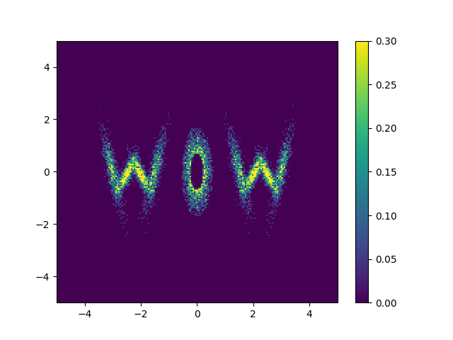
\[\begin{align} \mathcal{L}(\theta) = D_{KL}(q(\mathbf{x} \vert \mathbf{\theta}) \vert\vert p(\mathbf{x})) = \mathbb{E}_{q(\mathbf{x}\vert\vert\mathbf{\theta})}[\log q_\mathbf{x}(\mathbf{x}\vert \mathbf{\theta}) - \log p_\mathbf{x}(\mathbf{x})]. \end{align}\]But we could similarly, but not equivalently as the KL divergence isn’t symmetric with respect the input distributions, flip the order of the distributions and calculate our monte carlo averages using samples from the exact distribution. Let’s say I have samples from the distribution that I’m trying to approximate \(\mathbf{x} \sim p_\mathbf{x}(\mathbf{x})\), e.g. the samples below.
Or specifically looking at the approximate binned sample densities.
Then we could switch the input distributions to the KL divergence,
\[\begin{align} \mathcal{L}(\theta) = D_{KL}(p(\mathbf{x}) \vert\vert q(\mathbf{x} \vert \mathbf{\theta})) = \mathbb{E}_{p(\mathbf{x})}[\log p(\mathbf{x}) - \log q_\mathbf{x}(\mathbf{x}\vert \mathbf{\theta})]. \end{align}\]Expanding this out we can then observe something interesting,
\[\begin{align} \mathcal{L}(\theta) = \mathbb{E}_{p(\mathbf{x})}[\log p(\mathbf{x})] - \mathbb{E}_{p(\mathbf{x})}[\log q_\mathbf{x}(\mathbf{x}\vert \mathbf{\theta})], \end{align}\]looking at the first term, it does not involve the parameters that we are training \(\mathbf{\theta}\) at all, so it is effectively a constant.
\[\begin{align} \mathcal{L}(\theta) = C - \mathbb{E}_{p(\mathbf{x})}[\log q_\mathbf{x}(\mathbf{x}\vert \mathbf{\theta})] \end{align}\]And additionally the operation \(\mathbb{E}_{p(\mathbf{x})}\) can be calculated by the average of the approximate distribution \(q(\mathbf{x}\vert \mathbf{\theta})\) over the samples of \(p(\mathbf{x})\) that we theoretically already have. Again, the exact distribution is fixed from the perspective of our training and doesn’t change with respect to \(\mathbf{\theta}\).
\[\begin{align} \mathcal{L}_{\textrm{effective}}(\theta) \approx - \frac{1}{N} \sum_i^N \log q_\mathbf{x}(\mathbf{x}_i\vert \mathbf{\theta}) \end{align}\]This is an much easier loss function to optimise and we can cook up a training function pretty quick.
import tqdm
import numpy as np
from copy import deepcopy

def train(model, data, epochs = 100, batch_size = 256, lr=1e-3, prev_loss = None):

    # Not part of the flow, just making the samples we have nicely PyTorch compatible
    train_loader = torch.utils.data.DataLoader(data, batch_size=batch_size)

    # Standard optimiser
    optimizer = torch.optim.Adam(model.parameters(), lr=lr)

    # Storing the loss function values
    if prev_loss is None:
        losses = []
    else:
        losses = deepcopy(prev_loss)


    with tqdm.tqdm(range(epochs), unit=' Epoch') as tqdm_bar:
        epoch_loss = 0
        for epoch in tqdm_bar:

            for batch_index, training_sample in enumerate(train_loader):


                ############################
                ############################
                ### ACTUAL STEPs
                # ACTUAL STEP feeding the samples into the approximate distribution
                log_prob = model.log_probability(training_sample)

                # ACTUAL STEP take the negative mean as above
                loss = - log_prob.mean(0)

                # End of math/discussed steps
                ############################
                ############################

                # clear the previous gradients
                optimizer.zero_grad()

                # do backwards propagation
                loss.backward()

                # take a step with the optimiser
                optimizer.step()

                epoch_loss += loss

            epoch_loss /= len(train_loader)
            losses.append(np.copy(epoch_loss.detach().numpy()))
            tqdm_bar.set_postfix(loss=epoch_loss.detach().numpy())

    return model, losses
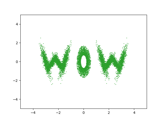
Actually implementing this, we can feed whatever samples we want into this, in my case I’m putting in some 2D samples that look like ‘WOW’.
torch.manual_seed(2)
np.random.seed(0)

num_flow_layers = 8
hidden_size = 32

NVP_model = RealNVPFlow(num_dim=2, num_flow_layers=num_flow_layers, hidden_size=hidden_size)
trained_nvp_model, loss = train(NVP_model, wow_samples, epochs = 600, lr=1e-3)
And then maybe repeat that final line with different learning rates/batch sizes a few times to get a nice plateau in the loss.

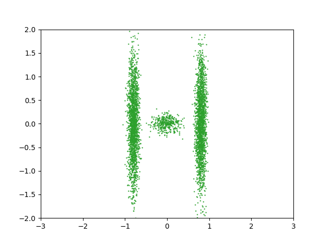
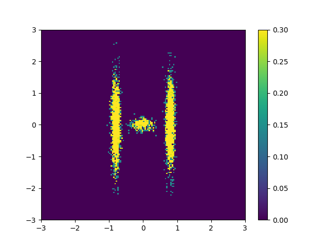
And looking at the result along with some samples that look like HELLO because why not.
Approximating an unknown unnormalised distribution
Going back to variational inference now, as a reminder our loss function is calculated with KL divergence below,
\[\begin{align} \mathcal{L}(\theta) = \mathbb{E}_{q(\mathbf{x}\vert\vert\mathbf{\theta})}[\log q_\mathbf{x}(\mathbf{x}\vert \mathbf{\theta}) - \log p_\mathbf{x}(\mathbf{x})]. \end{align}\]Similar to above, we can calculate the average using samples of the approximate distribution except the derivatives would be over the averaging samples as well. So, we will specifically draw samples from the base distribution of the flow, moving the transformation into the arguments of the averages not the averages themselves.
\[\begin{align} \mathcal{L}(\theta) &= \mathbb{E}_{q(\mathbf{x}\vert\vert\mathbf{\theta})}[\log q_\mathbf{x}(\mathbf{x}\vert \mathbf{\theta}) - \log p_\mathbf{x}(\mathbf{x})] \\ &= \mathbb{E}_{q(\mathbf{u})}[\log q_\mathbf{x}(T(\mathbf{u} \vert \mathbf{\theta})\vert \mathbf{\theta}) - \log p_\mathbf{x}(T(\mathbf{u}\vert\mathbf{\theta}))] \\ \end{align}\]There are some smarter ways to further manipulate this, but this will do for us for now. Let’s make up our new training function. Again, following the math pretty closely the specifics of the implementation are quite simple.
import tqdm
import numpy as np
from copy import deepcopy

def dist_train(approx_model, dist_to_approx, approx_samples=500,
                    epochs = 100,
                    batch_size = 256,
                    lr=1e-3, prev_loss = None):
    optimizer = torch.optim.Adam(approx_model.parameters(), lr=lr)

    if prev_loss is None:
        losses = []
    else:
        losses = deepcopy(prev_loss)

    base_dist_samples = approx_model.distribution.sample((int(approx_samples),))

    #####################
    #####################
    # Load the base dist sample into a dataloader
    #####################
    #####################

    train_loader = torch.utils.data.DataLoader(base_dist_samples, batch_size=batch_size)

    with tqdm.tqdm(range(epochs), unit=' Epoch') as tqdm_bar:
        epoch_loss = 0
        for epoch in tqdm_bar:
            for batch_index, training_sample in enumerate(train_loader):

                #####################
                #####################
                # Transform the base dist samples with the current iteration of the flow
                transformed_samples = approx_model.transform(training_sample)

                # Feed the transformed base dist samples into the current iteration of the flow
                realnvp_model_log_prob = approx_model.log_probability(transformed_samples)

                # Feed the transformed base dist samples into the exact (unnormalised) distribution to model
                exact_dist_log_prob = dist_to_approx(transformed_samples)

                # Take the average of the difference
                loss = (realnvp_model_log_prob-exact_dist_log_prob).mean()
                #####################
                #####################

                optimizer.zero_grad()
                loss.backward()
                optimizer.step()

                epoch_loss += loss
            epoch_loss /= len(training_sample)
            losses.append(np.copy(epoch_loss.detach().numpy()))
            tqdm_bar.set_postfix(loss=epoch_loss.detach().numpy())

    return approx_model, losses
To test this I’ll make up an annoying distribution for typical samplers such as something akin to the double moon distribution.
double_moon_radii_dist = dist.Normal(loc=1, scale=0.1).log_prob

def double_moon_dist(x):
    above_slice = x[:, 1]>0
    below_slice = x[:, 1]<=0
    x[above_slice, 0] = x[above_slice, 0] +0.5
    x[below_slice, 0] = x[below_slice, 0] -0.5


    radii = torch.sqrt(torch.sum(x**2, dim=1))

    return double_moon_radii_dist(radii)
Which we can plot.
pseudo_axis = torch.linspace(-4, 4, 161)
pseudo_samples = torch.vstack([mesh.flatten() for mesh in torch.meshgrid(pseudo_axis, pseudo_axis, indexing='ij')]).T


fig, ax = plt.subplots(1, 1, figsize=(5, 5))
pcm = ax.pcolormesh(pseudo_axis, pseudo_axis, double_moon_dist(pseudo_samples).reshape((len(pseudo_axis), len(pseudo_axis))).exp().T)
plt.colorbar(pcm, ax=ax)

Notably, this is not normalised correctly, and does not need to be, as the subsequent constant that this would incur on the log loss is not modified by the parameters of the approximation distribution that we are training. Chucking our model into our new training function, let’s see how well it does.
torch.manual_seed(2)
np.random.seed(0)

num_flow_layers = 8
hidden_size = 32

NVP_model = RealNVPFlow(
    num_dim=2, num_flow_layers=num_flow_layers, hidden_size=hidden_size)

dist_trained_nvp_model, loss = dist_train(
    NVP_model, dist_to_approx=double_moon_dist, approx_samples=5000,
    epochs = 100, lr=1e-3, batch_size=1024)

dist_trained_nvp_model, loss = dist_train(
    NVP_model, dist_to_approx=double_moon_dist, approx_samples=5000,
    epochs = 100, lr=3e-4, batch_size=1024, prev_loss = loss)

dist_trained_nvp_model, loss = dist_train(
    NVP_model, dist_to_approx=double_moon_dist, approx_samples=5000,
    epochs = 100, lr=1e-4, batch_size=1024, prev_loss = loss)

Conclusion
So in this post we:
- Learnt how to make our own implementation of a RealNVP normalising flow from scratch (using PyTorch)
- How to train this normalising flow model to approximate a given sample distribution
- How to train this normalising flow model to approximate an unnormalised probability distribution
Hopefully, I wrote this in such a way that each step was super easy, if not, feel free to shoot me an email and I’ll respond as soon as I’m near a computer. For further resources I again want to emphasize heading over to Eric Jang’s website specifically the posts that I am borderline copying e.g. Normalizing Flows Tutorial, Part 1: Distributions and Determinants. And to give Normalizing Flows for Probabilistic Modeling and Inference a read if you weren’t already, I basically just cover bits and pieces from that, and then you can implement more state-of-the-art (but still pretty simple) normalising flow models.
Extra: 09/08/2025
Just for another example of how expressive RealNVP can be despite it’s simplicitly, using samples from the scikit-learn package’s make_swiss_roll function, we can also see that the method can handle higher dimensions with a couple slight tweaks. Specifically just the cell specifiying the dimension
torch.manual_seed(2)
np.random.seed(0)

num_flow_layers = 8
hidden_size = 32

NVP_model = RealNVPFlow(
               num_dim=3,
               num_flow_layers=num_flow_layers,
               hidden_size=hidden_size)
trained_nvp_model, loss = train(
                             NVP_model,
                             torch.tensor(sr_points),
                             epochs = 500,
                             lr=1e-3)
Then with the same training I was able to get the below GIF!

In log-space, which we often work in for the sake of numerical instability it becomes the even simpler sum! ↩