In this post I will attempt to give an introduction to binary classifiers and more generally neural networks.

Resources

Hey there, this is another introductory post, going into binary classifiers and kinda neural networks in general. Figured it would be nice to have alongside all the other things in my posts that rely on neural networks that at least gives an intuitive feel for how neural network work and for a future post where you can use binary classifiers to perform likelihood-free or simulation-based inference with Nested Ratio Estimation.

As usual, here are some of the resources I’m using as references for this post. Feel free to explore them directly if you want more information or if my explanations don’t quite click for you:

• 3Blue1Brown’s series on neural networks
• StatQuest with Josh Starmer’s intro video on neural networks and his subsequent neural networks playlist
• An introduction to Neural Networks for Physicists by G. Café de Miranda, Gubio G. de Lima, and Tiago de S. Farias (possibly biased by the fact that I am a physicist)
• An introduction to artificial neural networks by Coryn A.L. Bailer-Jones, Ranjan Gupta, and Harinder P. Singh

Table of Contents

• Motivation
• Generating The Data
• The Multilayer Perceptron
• The Loss Function
• The Optimizer
• Training
• Evaluation
• Model Applicability
• Further Reading

Motivation

Many problems in real life can be boiled down to a yes or no question: “AI or not AI?”, “Dog or Cat?”, “Cancerous or not cancerous?” or “Cake or not Cake?”

The modelling of this kind of problem falls under the umbrella of logistic regression or binary classification. Here we will focus on thinking of the problem from a binary classification lens. One of the most common uses of machine learning/neural networks is to handle this kind of problem, showing how this is done is the goal of this post.

We will use a simple example of 1D data that either comes from one of two normal distributions, and see how we can train a neural network to do this separation and the limitations of this.

(If you want to run the code in this tutorial on your own computer you will just require the packages PyTorch, numpy and matplotlib.)

Generating The Data

Let’s say we want 10,000 samples and that the standard deviation of the two groups is the same at 0.2. With means 1.0 and 2.0 respectively.

# A machine learning package
import torch
# The torch.distributions has a lot of useful distributions including the normal and poisson distributions
from torch.distributions.normal import Normal

# The "seed" here is a number that the computer uses to generate pseudo-random numbers
    # Fixing this number means that the results of this notebook will stay consistent.
    # Feel free to change it and see this in action (just some of my text won't be 100% correct)
torch.manual_seed(0)

# ----- Generate data -----
num_samples = int(1e4)
scale = 0.2

true_params = {'a': 1.0, 'b': 2.0}

a_samples = Normal(loc=true_params['a'], scale=scale).sample((num_samples,))
b_samples = Normal(loc=true_params['b'], scale=scale).sample((num_samples,))

Let’s have a look at these samples using matplotlib

from matplotlib import pyplot as plt

# making a fake axis so that the scale of the bins is the same for the two groups
    # and so that it adjusts itself if you want to change the means of scales later on
pseudo_axis = torch.linspace(
    min([true_params['a'], true_params['b']])-5*scale,
    max([true_params['a'], true_params['b']])+5*scale,
    101
    )

fig, ax = plt.subplots(1,1, figsize=(5,4))
ax.hist(a_samples, bins=pseudo_axis, label='a', alpha=0.8)
ax.hist(b_samples, bins=pseudo_axis, label='b', alpha=0.8)
ax.set(
    xlabel='X',
    ylabel='Number of samples'
)
ax.legend()
plt.show()

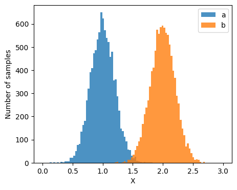
Where I’ve designated the general variable for the samples as ‘X’. Combining the two as such…

X_samples = torch.cat([a_samples, b_samples]).unsqueeze(1)  # shape: [2*num_samples, 1]
X_labels = torch.cat([torch.zeros(num_samples), torch.ones(num_samples)]).unsqueeze(1)  # shape: [2*num_samples, 1]

While combining the samples we’ve also created a new piece of information called X_labels, this tells us whether a sample from ‘X’ is either from ‘a’ (=0) or ‘b’ (=1). The reason that we use 0 and 1 instead of ‘a’ and ‘b’ as the labels is essentially that computers (especially PyTorch) prefer working with numerical quantities (what we’ve specifically done is similar to one-hot-encoding).

We will then further augment our data to work nicely with the Python package PyTorch. In almost all classification tasks you have a set of inputs, X_samples, and a 1D set of labels y_labels and hence you can use this same general setup for whatever (similar) problem you wish.

One particular thing that this augmentation does is split the data into ‘batches’ which are small segments of the data that are utilised together at a single time. We want to include as many of these together at once without exceeding our computer’s RAM. In our case we’re dealing with 1D data so it isn’t that much of a concern, but if you were dealing with 1000s of 256x256 images, you would really need some batching.

from torch.utils.data import TensorDataset, DataLoader

# ----- Dataset & DataLoader -----
dataset = TensorDataset(X_samples, X_labels)
loader = DataLoader(dataset, batch_size=256, shuffle=True)

We’ve additionally shuffled our data so that the classifier doesn’t just figure out that the first half of the data is from group ‘a’ and the second half is from group ‘b’ because we want it to actually learn whether the samples themselves look like they’re from group a or b.

The Multilayer Perceptron

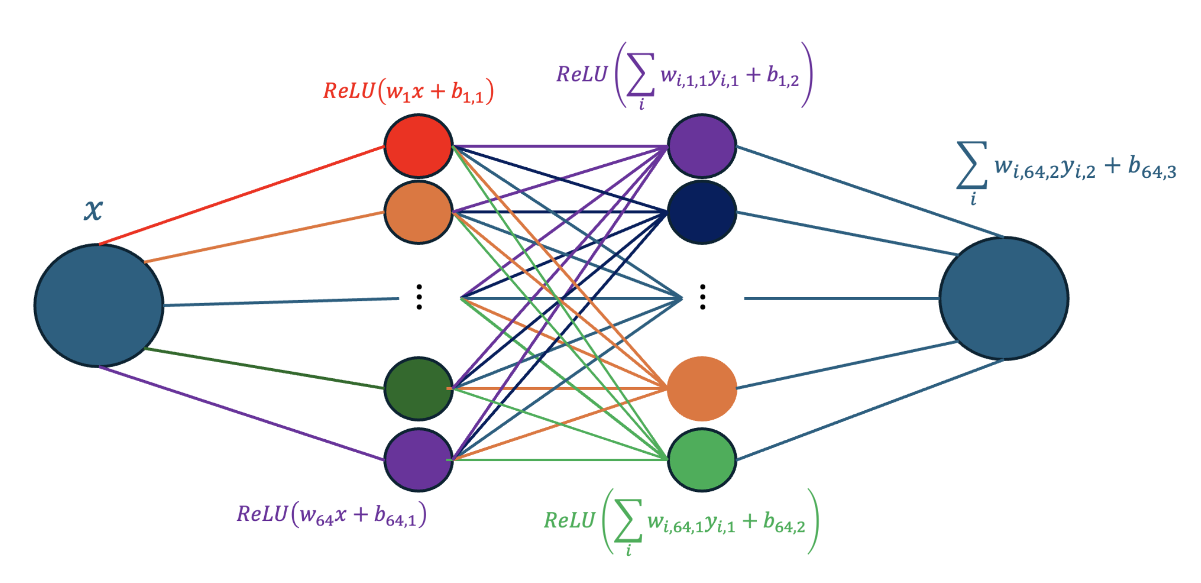
We then want to setup our machine learning classifier! We’re going to set up a basic neural network or MLP. We will use 3 layers that involve input values \(y_i\) (e.g our X samples or the outputs of the previous layers), bias terms \(b\), weights \(w_i\) and activation functions \(f\) (specifically ReLU) each of which work as,

import torch.nn as nn
import torch.nn.functional as F

# ----- Network -----
class Net(nn.Module):
    def __init__(self):
        super().__init__()

        # First layer that takes 1D X input and spreads it across 64 nodes
        self.fc1 = nn.Linear(1, 64) 

        # Second layer that takes output of previous layer and spreads it across 64 new nodes
        self.fc2 = nn.Linear(64, 64)

        # Third layer that takes output of previous layer and condenses it into a single node
            # that indicates either a=0 or b=1
        self.fc3 = nn.Linear(64, 1)


    def forward(self, x):

        # Take output of weights * x + bias and feed it into the activation function
        y = F.relu(self.fc1(x))

        # Take output of weights * y + bias and feed it into the activation function
        y = F.relu(self.fc2(y))

        # Take output of weights * x + bias and DOES NOT feed into activation function
            # as the loss function we are working with presumes this kind of "logit"
        return self.fc3(y)  # no sigmoid here

net = Net()

This is a little abstract though so here’s the structure of the network a little more graphically definitely not screenshotted from PowerPoint.

We then need to construct a function that tells the neural network how well it’s doing and another one to tell it how to do better.

The Loss Function

The function that we use to tell how well the neural network is doing is called BCEWithLogitsLoss standing for ‘Binary Cross Entropy with Logits Loss’. Binary cross entropy is a specific application of cross-entropy.

# ----- Loss  -----
criterion = nn.BCEWithLogitsLoss()  # logits + binary labels

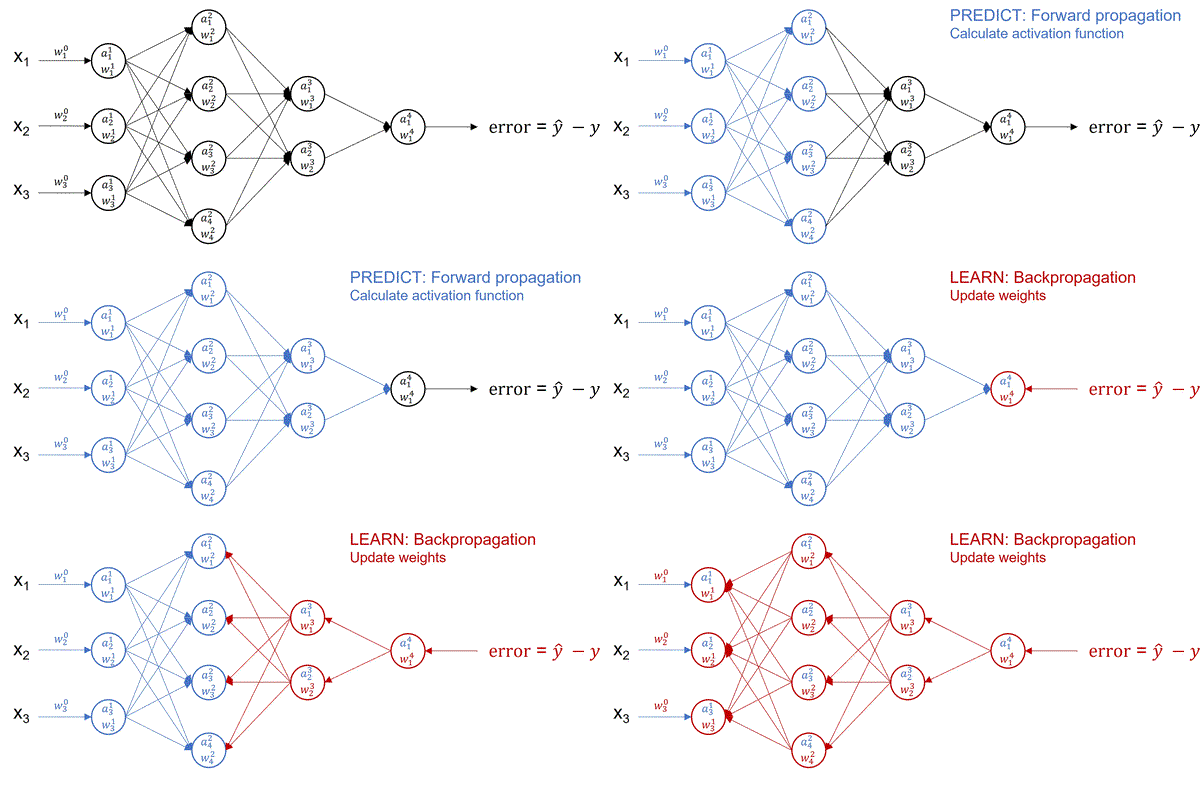
The flow of evaluation and correction of a neural network can be seen in this GIF, and if you want to know how this actually works I’d recommend this video (StatQuest again, guy’s great, intro’s are not).

Binary cross entropy is defined as,

where \(N\) is the number of training samples (in our case \(10^4\)), \(y_i\) the actual labels and \(p_i\) the probability of the value being 0. If we had a perfect classifier then when \(p_i=0\) then \(y_i=0\) and when \(p_i=1\) then \(y_i=1\). You can see that when this extreme is satisfied then \(BCE=0\) and is otherwise \(>0\). So as the training persists we want this value to go down towards zero.

The binary cross entropy is a specific case of the more general cross entropy, described as,

where in BCE \(y_i\sim q(y\vert x)\) and here \(p(y\vert x, \theta)\) denotes the probability of label \(y\) given input \(x\) and model parameters \(\theta\). This more general equation over \(y\) allows for more possible outcomes, the binary cross entropy being the result with just two outcomes such that \(p(y=0\vert x, \theta) = 1-p(y=1\vert x, \theta)\).

In these kind of problems (and very generally in inference tasks) we often wish to minimise the ‘distance’ between an exact distribution (e.g. a posterior) and our approximate distribution. This is almost always done with the KL divergence¹. Following this we may want to blindly apply it here,

During our optimisation, the only thing that we can change is \(\theta\), we are given our example \(x\) and \(y\) as inputs and outputs, so we can’t really change the first term and hence it would be a waste of computations to calculate it. And voila, the remaining term (including minus sign) is then our cross entropy.

For another perspective (although it is almost exactly the same), I liked this video.

The Optimizer

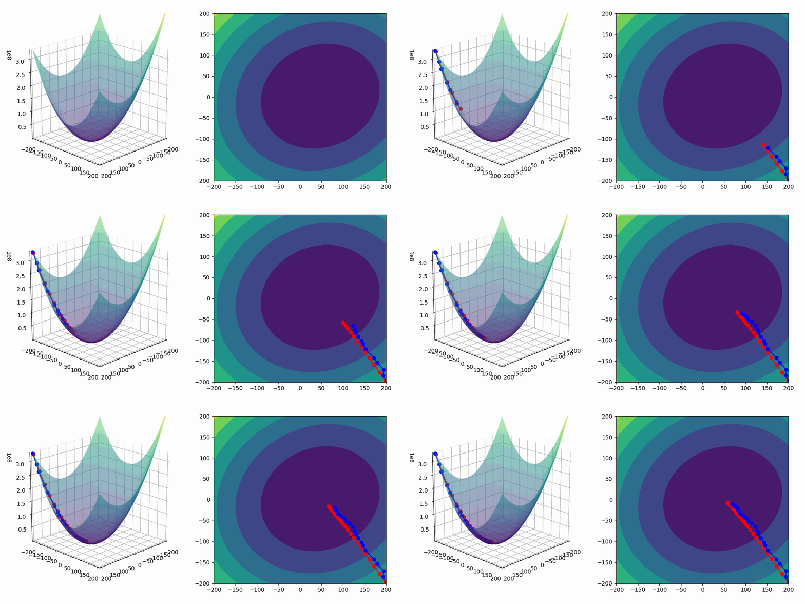
The function that we use to update our neural network, or tell it how to do better during the training/minimise our loss function, is SGD or Stochastic Gradient Descent which if you image our loss as the bottom of a valley, gradient descent will allow us to use information about how steep the valley is rather than having to learn that information by randomly moving around, and stochastic because it uses random subsets of the data to calculate the gradients to minimise memory load among other reasons.

# ----- Optimizer  -----
optimizer = torch.optim.SGD(net.parameters(), lr=0.01)

In the GIF below you can imagine that our loss is the shape the dots are traversing, in red is if we use an optimiser with gradient descent that uses all the data, giving us exact gradients (but may be computationally expensive) and in blue our stochastic gradient descent, which gives us noisier estimates of the gradient but is much less computationally expensive.

Training

Now that we have that it’s just a question of how to train the neural network, a big part of that is backpropagation which is nicely explained here after you suffer through the intro or this video then this video from the goat 3Blue1Brown if you want other sources for how it works.

My TLDR, is that in supervised training, where you have the outputs for the relevant inputs in your training data, we know what our final answer should be, and we can calculate gradients relating to our weights and biases to move the final output layer (in our case just single output) to look more like the correct output. e.g. If our output says that the probability of the our input coming from group b/=1 is 0.7 and it is actually from group b, then we need to maximise the weights of the nodes that increase our output value and minimise the values of the weights that decrease it. You then follow that backward through the network propagating the derivatives via the chain rule, hence backpropagation.

# ----- Training Loop -----
losses = []
for epoch in range(70):
    running_loss = 0.0
    for inputs, labels in loader:
        optimizer.zero_grad() # Clear old gradients from the previous loop
        outputs = net(inputs) # Evaluate the model on the training data
        loss = criterion(outputs, labels) # See how badly the neural did based on the labels of the data
        loss.backward() # perform backpropagation
        optimizer.step() # change the weights and biases to make the neural network better
        running_loss += loss.item() # keep track of loss values
        losses.append(loss.item()) # keep track of losses for later use in plotting

    if (epoch+1) %10 ==0:
        print(f"[Epoch {epoch+1}] Loss: {running_loss/len(loader):.4e}")

print("Finished Training")

We can then look at our loss, something telling us how well our neural network is doing overall, as a function of the iterations of the training.

from matplotlib import pyplot as plt

plt.figure()
plt.plot(losses)
plt.xlabel("Iteration")
plt.ylabel("Loss")
plt.yscale('log')
plt.show()

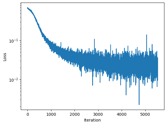
By the fact that this has basically plateued we can say that the neural network won’t noticeably improve/do any better even if we run it for way longer.

Evaluation

Now let’s see how well it practically does against some new data generated from the same distributions.

a_test_samples = Normal(loc=true_params['a'], scale=scale).sample((num_samples,))
b_test_samples = Normal(loc=true_params['b'], scale=scale).sample((num_samples,))

X_test_samples = torch.cat([a_test_samples, b_test_samples]).unsqueeze(1)  # shape: [2*num_samples, 1]
X_test_labels = torch.cat([torch.zeros(num_samples), torch.ones(num_samples)]).unsqueeze(1)  # shape: [2*num_samples, 1]


with torch.no_grad(): # no grad means we're telling PyTorch we don't need to keep track of gradients for this bit

    
    preds = torch.sigmoid(net(X_test_samples))
    predictions = (preds > 0.5).float()
    accuracy = (predictions == X_test_labels).float().mean()
    print(f"Accuracy: {accuracy.item()*100:.5f}%")

And if you didn’t change the manual seed line at the top of the script you should see that the neural network is 99.355% accurate! Meaning if we threw ~1000 samples at the neural network it would only guess ~<7 incorrectly.

Now I’m just going to re-run everything above but changing the number of samples that we use to train the neural network and the scale of the distributions to see how the neural network does.

Model Applicability

And if you didn’t change the manual seed line at the top of the script you should see that the neural network is 99.355% accurate! Meaning if we threw ~1000 samples at the neural network it would only guess ~<7 incorrectly.

Now I’m just going to re-run everything above but changing the number of samples that we use to train the neural network and the scale of the distributions to see how the neural network does. We would naturally expect worse results (low distinguishability) for larger scales because the distinction between the samples would be naturally harder, and worse results for smaller training sets because we give less information for the classifier to work off of.

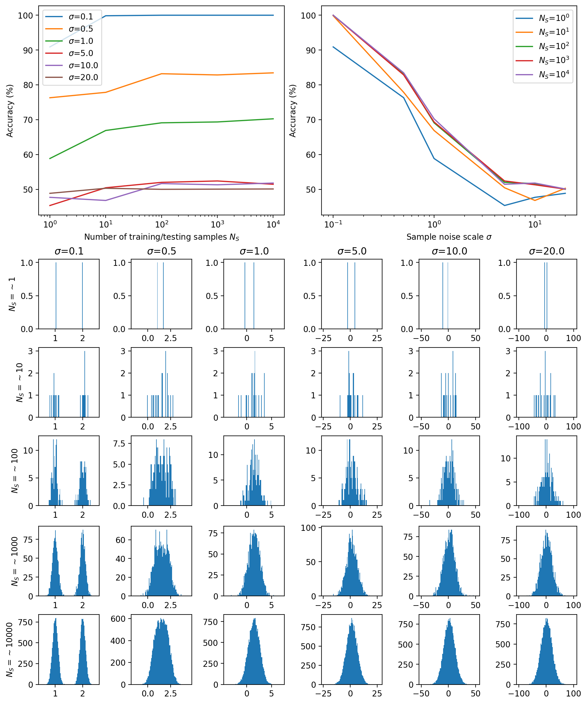
You can see both of these changes on the samples above but the impact of the scaling is much greater. When looking at the samples directly and comparing to the performance as can be seen below you can intuit that this should be the case presuming that our classifier is doing the most it can with the data provided. I don’t know about you, but after \(\sigma \approx 1.0\) I couldn’t even say that there were two gaussians there, yet alone which samples came from which one, so it makes sense that the neural network similarly starts losing it’s distinguishing power.

Conclusion

A key note to remember here at the end of the day though is that neural networks (that aren’t just a small number of nodes e.g. \(\sim 10\)) are often what we call a ‘black boxes’. We don’t exactly know how or why they can do what they do. In fact, the interpretability or knowing why neural networks (specifically LLMs) can even do some of the things that we ask them to do is an open question (e.g. here for a paper on the topic or here for a video by Alberta Tech).

For the purposes of this task, all we need to know is that the neural network is some sort of function with a bunch of parameters and we train these parameters so that the output of the function correctly guesses whether an input comes from group ‘a’ or group ‘b’.

In a future post I may go into more detail about how backpropagation of neural networks works rather than my handwave argument above.