In this post I will attempt to give an introduction to variational inference with some examples using the NumPyro python package. Partly under construction

Hey there, this is more of an introductory post than my last if you’re following along. I gave a quick explainer in my normalising flows post on variational inference, but I figured I’d do a standalone post on it, talk about other methods within the field and more detailed fundamentals. I’m definitely going to miss some useful framework somewhere, so please email me if you have any suggestions.

As usual, here are some of the resources I’m using as references for this post. Feel free to explore them directly if you want more information or if my explanations don’t quite click for you:

• Variational Inference: A Review for Statisticians - David M. Blei, Alp Kucukelbir, Jon D. McAuliffe
• Stochastic Variational Inference - Matt Hoffman, David M. Blei, Chong Wang, John Paisley
• Variational Inference: ELBO, Mean-Field Approximation, CAVI and Gaussian Mixture Models - Bruno Magalhaes
• VI - 6.1 - CAVI - Coordinate Ascent VI - Meerkat Statistics
• Black Box Variational Inference - Ranganath, Gerrish, Blei
• Rao Blackwell Theorem - Statistics Curiosity
  • I could not find a source that explained this concept simply but in detail in under 2 hours, except for this guy. Love you man
• Black Box Variational Interference – Rajesh Ranganath
• Automatic Differentiation Variational Inference - Kucukelbir, Tran, Ranganath, Gelman, Blei
• Reparameterization Trick - Wikipedia (Yes Wikipedia)
• The Reparameterization Trick - Emma Benjaminson (for some different distributions’ tricks)

Table of Contents

• Motivation
• Core Idea
• Mean Field Approximation and CAVI
• Black Box Variational Inference
  • Rao-Blackwellisation
  • Control Variates
• But I can’t be bothered taking derivatives… could I do them automatically? - ADVI
• Limitations
• Further Reading
• Appendices

Motivation

In short, variational inference approximates a complex target distribution (like a Bayesian posterior) using a pre-defined set of distributions, and chooses the best within the set by solving an optimization problem. This leads to the fact that the target distribution will not be within the set (and is often actually assumed not to be a priori). So, why are people so interested/why am I discussing variational methods if it’s a given that it won’t give you your target distribution? In short, MCMC is hard and variational inference can be less hard and still give you something reasonable.

In particular, despite the overwhelming success of MCMC methods when it comes to Bayesian inference they do not scale for high dimensional distributions (often called p problems) or for extremely large and/or high dimensional sets of data (often called n problems).

Variational Inference (which I will now denote VI) turns all of this into an optimisation problem and thus can utilise many of the tools of optimisation such as automatic differentiation and stochastic optimisation methods. Allowing VI methods to more easily scale for n and/or p problems.

Additionally, VI can more easily update an approximate distribution with new data conditioned on previous data. Done by using the previous version of the distribution from the original set of data as a starting distribution, and simply updating the loss function with the new data. Similar to a stochastic optimisation method of tempered annealing. (If this doesn’t make sense, I go more into depth once we have a loss function to actually optimise.)

Perhaps most importantly: VI provides a parametric representation of the posterior, rather than a set of samples. This is especially valuable in settings where you need to manipulate or compose distributions, such as in probabilistic programming or generative modeling (e.g., VAEs) or more specifically, to use as a prior for future inference.

Okay then — what are the core ideas behind VI? How can you implement it yourself, and what should you watch out for if you do? I’m focusing on bayesian inference, hence from here I’ll stop talking about ‘target distribution’ and instead ‘posterior’ for convenience. But of course, you can do a quick replacement as the posterior is just a distribution.

Core Idea

The key idea here is, that you have an approximate distribution that you can sample relatively quickly with a set of parameters controlling its shape, and you want to optimise these parameters to make the shape of the approximate distribution as close to the shape of the posterior as possible. More abstractly, if you are within a space of distributions within which the set of approximate distributions and your posterior are, you want the distance between your posterior and your approximate distribution to be minimised.

Unfortunately, it is not standard to measure “distance” between two distributions, but to use a “divergence”¹, which is pretty close but not quite. If you have a distribution \(X\) and distribution \(Y\), a function that would quantify the distance \(d\) between them would satisfy symmetry \(d(X, Y)=d(Y, X)\). i.e. In real world settings, if I run 5km North, then run 5km South, I should be in the same direction I started (and quite tired from the running). But for a divergence \(D\), then \(D(X, Y)\neq D(Y, X)\). i.e. If I run 5km North, then run 5km South, I don’t necessarily end where I start (and now likely dying from dehydration because I always forget to drink water on my runs). That said, divergences do tell us something important: if two distributions are identical, the divergence between them is zero. And the more dissimilar they are, the larger the divergence tends to be — regardless of which one you start from².

The overwhelming most common way that we measure the divergence between two distributions in statistics is the Kullback-Leibler divergence, denoted \(KL(q\mid\mid p)\) for two distributions \(p\) and \(q\). For these two distributions over a discrete sample space \(\mathcal{Z}\) then the Kullback-Leibler divergence is defined,

And in a continuous setting,

In either case, you can see that these are an average of \(\log \frac{q}{p}\) over the given sample space. If the two distributions are the identical, then \(\frac{q}{p}=1\), the \(\log\) will give 0 everywhere, and the average over anything of 0 is 0.

Note that KL divergence is not symmetric — in general, \(KL(q \,\|\, p) \neq KL(p \,\|\, q)\) — which reflects the asymmetry we talked about earlier¹.

These divergences are usually estimated using Monte Carlo sampling on \(\log \frac{q}{p}\). For those unfamiliar: you sample from the distribution over which you’re averaging (in this case, \(q(z)\)), and plug those samples into the function of interest — here, \(\log \frac{q(z)}{p(z)}\). Since you’re taking a weighted average over a finite set of \(N\) samples, it behaves much like the discrete version of KL anyway.

Going back to the goal of this post, minimizing the divergence between an approximate distribution and a posterior. If we think of \(p(z)\) as our posterior and \(q(z)\) as our approximation, then apriori we would need a functional form of our posterior… which is meant to be the goal³?

Well what we’re going to do is slightly manipulate the \(KL\) divergence to get something practical to use and still representative of the divergence. If we split up the posterior into it’s constituent parts according to Bayes’ theorem (simultaneously introducing the posterior’s dependence on data \(x\)) we find,

Where we were able to take out the evidence \(p(x)\) as it has no dependence on \(z\) hence is essentially a constant within this average. Remembering that we are trying to make \(q(z)\) look like \(p(z\mid x)\), then any kind of optimisation will not involve \(p(x)\) as it doesn’t involve \(q(z)\). So we define the ELBO,

ELBO stands for Evidence Lower BOund, because by a quick rearrangement of the above you can see,

As the KL divergence positive definite, the ELBO is a lower bound for \(p(x)\). AND, as previously stated, the ELBO works as the target for our optimisation, we maximise the ELBO and subsequently minimise the KL divergence. In practice, we don’t compute the ELBO exactly — we estimate it using samples, and we adjust the parameters of \(q(z)\) to maximize it.

Mean Field Approximation and CAVI

The question is then how do we go about maximising the ELBO? Well for that I’m first going to introduce a simple framework under which you can construct sets of distributions to optimise over, the Mean Field Approximation. The approximation is that the variables of the approximate distribution factorise. Meaning that if you have a probability density \(q\) for your posterior over variables \(z=(z_0, z_1, ..., z_N)\) then we can represent \(q(z)\) as,

Where \(q_i\) represents a factorised probability over the \(i^{\text{th}}\) component of \(z\). If we make this factorisation such that each \(q_i\) is a gaussian, then we represent our posterior with a multivariate gaussian with no covariance. I have an example of this approximation here.

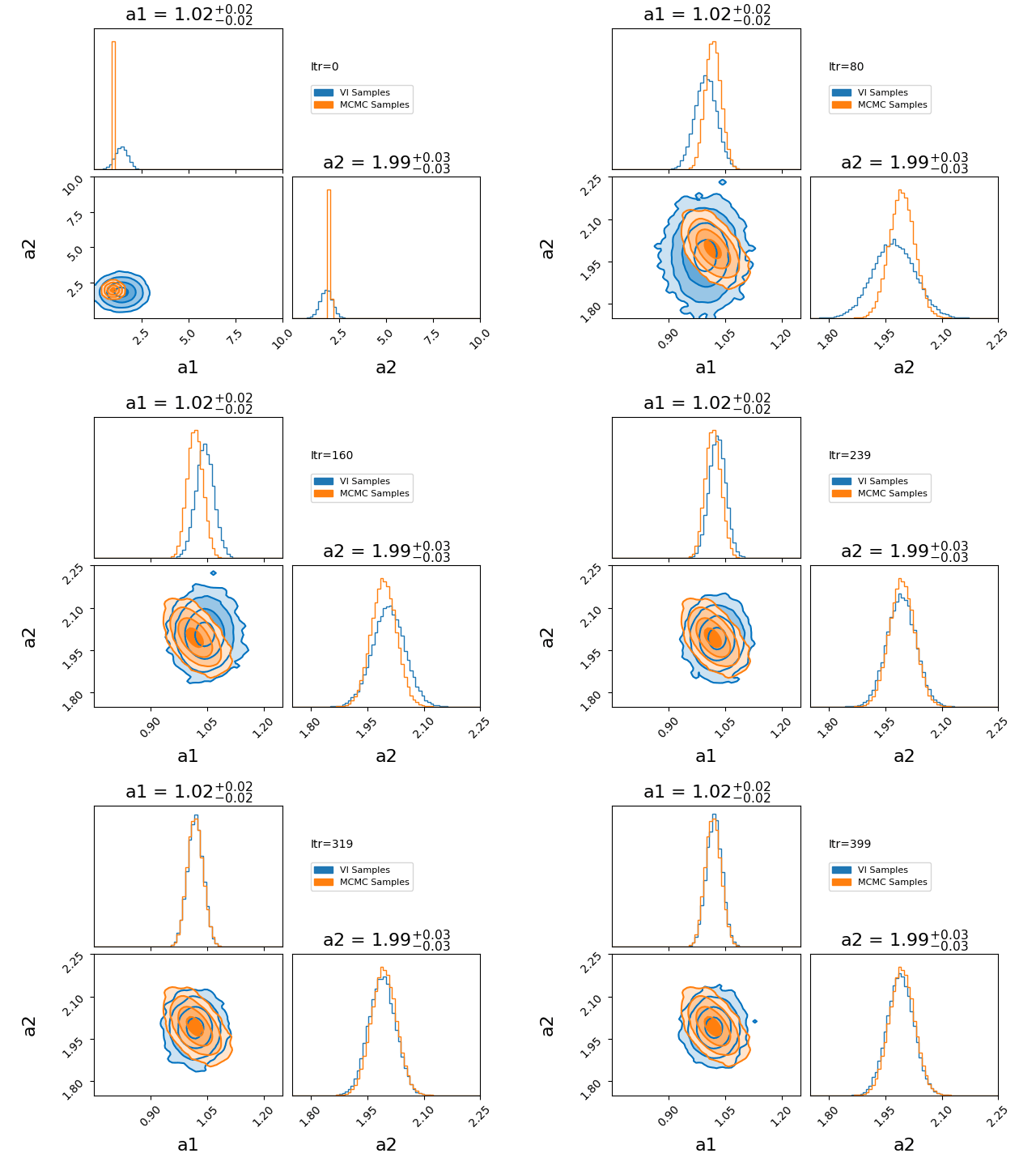
You’ll notice that the variational approximation is slightly more concentrated than the true posterior. This happens because, under the assumption of independent (mean-field) Gaussians, it is more optimal to concentrate around the high-density core of the posterior. Additionally, because we’re assuming single gaussians for our components there is no chance that using this will give any reasonable answer for a multi-modal problem. However, if you believe that your posterior will be roughly gaussian with a single mode in each dimension then the mean field approximation has its utility in being lightweight and has many established quick optimisation techniques.

How the optimisation in the GIF was done is the main topic of this section, it is called CAVI.

If we plug the general mean field approximate distribution into the ELBO we can isolate a given probability density component as follows.

We are then trying to maximise the ELBO while looking along a particular component, \(q_j\), and trying to maximise it with respect to that. And as is typical, we’re looking for a local maximum, so we set the derivative of the thing we’re trying to optimise over with respect to the thing we’re changing to 0. i.e.

Where \(\mathbb{E}_{q_{-j}}\) represents the average over all the components of \(q\) except the \(j^\text{th}\) and in the final couple of steps you will note that the \(1 - \sum_{i=0\neq j}^N \mathbb{E}_{q_{-j}}\left[ \log(q_i(z_i)) \right]\) has nothing to do with \(z_j\) or \(q_j\), so if we’re trying to optimise the form of \(q_j(z_j)\) then these are effectively constants and \(\exp(\text{constant})=\text{constant}=C\).

Now of course this form of \(q_j(z_j)\) cannot be calculated exactly in practice as it involves marginalising over all the other variables of interest, so CAVI assumes that the posterior satisfies conjugacy (i.e. the form of the prior and the likelihood has a known form typically following that of the prior). Without conjugacy, the expectation \(\mathbb{E}_{q_{-j}}\left[\log p(z, x) \right]\) becomes analytically intractable, so we can’t recover a closed-form expression for \(q_j(z_j)\).

So in summary, what CAVI does is isolates a given \(j^\text{th}\) component of your approximate distribution \(q_j(z_j)\) (which we can do under the mean field approximation) marginalise over the other components for every component of \(z\) except \(z_j\) to get an exact updated estimate for \(q_j(z_j)\).

The case of a gaussian mean field approximation to a posterior utilising a CAVI distribution is shown below. The blue distribution shows the variational approximation for a given iteration, while orange samples are from the MCMC posterior as a stand-in for the exact posterior.

Now CAVI is great because it doesn’t require derivation of gradients and is pretty stable, however, it only works for conjugate models with the mean field simplification…

Black Box Variational Inference

So if you don’t want to derive a model specific optimisation technique/can’t because it doesn’t satisfy conjugacy but still fine with taking the mean field approximation, a common alternative is Black Box Variational Inference or BBVI.

BBVI starts off with producing a generalised form for the gradient of the ELBO with respect to the general parameters of the approximating distribution which I denote \(\lambda\) (heavily inspired by arXiv:1401.0118)

We then note that \(\nabla_\lambda[\log p(z,x)]=0\) because \(p\) doesn’t involve \(\lambda\) in any way and the following,

Hence,

And in case it’s useful \(\nabla_\lambda \log q(z\mid\lambda)\) comes up in a few contexts and is often called the score function. If we then estimate this using monte carlo sampling of the variational approximation using \(S\) samples \(\sim q(z\mid\lambda)\) then,

Now this is great, we get a generalised form of gradients for use in our optimisation however, because it is estimated through a Monte Carlo estimate it is quite noisy. So what Ranganath and co did in their original paper was combine two methods to stabilise the estimate.

(You can skip the next two sub-sections if uninterested, they are there simply to stabilise the gradient estimate.)

Rao-Blackwellization

In their own words,

“Rao-Blackwellization (Casella and Robert, 1996) reduces the variance of a random variable by replacing it with its conditional expectation with respect to a subset of the variables.” - Ranganath et al.

Our goal is to calculate a less noisy estimate to update our parameters. Rao-Blackwellization lets us reduce the variance of our gradient estimator by computing a conditional expectation over some variables. In variational inference, we can apply this to reduce the noise in the estimate of the gradient with respect to one variational parameter by integrating out the others. First expanding out our exact formula for the gradient.

Isolating the \(i^\text{th}\) component,

Then assuming that the joint density isn’t something pathological such that you can separate terms/factors that involve \(z_i\) such that you can separate the joint density into terms \(p(z, x) = p_{i}(z_{(i)}, x) \cdot p_{-i}(z_{(-i)}, x)\), where \(p_{i}(z_{(i)}, x)\) represents all terms that involve \(z_i\) in the joint.

Everything in the very right term doesn’t depend on either \(z_i\), \(q_i\) or \(\lambda_i\) so they are effectively constants when trying to optimise in that component. A similar argument can be made for the average of the \(i\) components of the joint over the other components \(\mathbb{E}_{q_{-i}} \left[\log p_i(z_{(i)}, x)\right]\).

We can look at the variance for this kind of estimate, let’s say \(\hat{J}(X_i) = \mathbb{E}_{-i}[J(X_i, X_{-i})]\), where \(J(X_i, X_{-i})\) is the joint, and noting that \(\mathbb{E}[\hat{J}(X_i)] = \mathbb{E}[J(X_i, X_{-i})]\) then,

So no matter what, the variance of our new estimator is lower than our original, meaning less noisy.

Control Variates

Okay, so we’ve gotten a less noisy estimate for the \(i^\text{th}\) component of the gradient by swapping out the joint density with another variable that has the same expectation value but lower variance. We can further decrease the variance on our estimate using control variates. TLDR: A control variate is an auxiliary function with known expectation, used to reduce the variance of a Monte Carlo estimate.

As a quick intro, if I have some function \(f(z)\) of which I want to estimate the average of, I can instead look at another variable \(\hat{f}\) that has the same expectation value described as the following,

You can see that we’ve introduced another function \(h\) which doesn’t seem to do anything, and it doesn’t … to the average at least because,

However, it will impact the variance,

And then just because I didn’t remember this simplification while writing this, I note that,

Hence,

So, although we started with an arbitrary \(h(z)\) we may want to pick one that best minimises \(Var[\hat{f(z)}]\), i.e. one that has a high covariance with it \(Cov\left(f, h\right)\). In BBVI, our goal is to reduce the variance of the gradient of the ELBO. Since the score function \(\nabla_\lambda \log q(z\mid\lambda)\) appears in the gradient, it makes sense to use it as the control variate.

Hence, in terms of our covariate theory,

Now, your remaining question should be, what’s \(a\)? Well again, we want to minimise the variance in \(\hat{f}(z)\) as much as possible, so we will look for a minimum with respect to \(a\) by looking for when the derivative of the variance of \(\hat{f}(z)\) is 0.

Thus our final expression for the variance of the function \(\hat{f}(z)\) is,

I made a gif showing how much more efficient this algorithm is compared to CAVI but it looks exactly the same so I’ll save you the time. However, its still quite noisy despite these variance stabilisation methods, meaning that the step size has to be quite small, decreasing the rate of convergence.

But I can’t be bothered taking derivatives… could I do them automatically? - ADVI

Despite the increased generality of BBVI (doesn’t require conjugacy), if you have a highly multidimensional problem, calculating all the gradients of the variational density can be quite tedious (and again the estimates of the ELBO gradient can still be quite noisy). This motivates Automatic Differentiation Variational Inference (ADVI) — a method that automates much of the process using autodiff and the reparameterization trick.

In short, ADVI replaces hand-derived gradients with those computed via automatic differentiation: a system that tracks the computational graph of elementary operations (like +, *, log, exp) and uses the chain rule to compute exact gradients.

Instead of estimating the gradient of the ELBO with score functions (as in BBVI), ADVI reparameterizes the variational distribution so the gradient flows through the samples themselves, enabling lower-variance, faster-converging optimisation.

To make the derivatives more well-behaved in ADVI we transform any variables into a continuous domain (if everything already has \(\mathbb{R}\) support then \(T\) is an identity). If our exact joint target density is \(p(z, x)\) where \(z\) is constrained to some domain, then we apply \(T\) to find,

We then need to translate our target joint density and variational density to use these variables. Our joint density can be denoted,

Then similar to the original ADVI paper we will compare the performance of two variational gaussians approximations; one with a diagonal covariance matrix (mean field approximation) and a full rank covariance matrix (allowing us to actually look at correlations!).

For the mean field approximation we can describe the variational density which can be split into a product of gaussians in each of the K dimensions of interest,

And for the full rank gaussian,

Now, our loss can be expressed as,

If we wanted to compute the gradients of this, that can be quite difficult for the computer to handle due to the expectation being done over the variational density we are trying to optimise. So, we employ the reparameterisation trick (called elliptical standardization in the original paper) where we transfer the direct sampling of the variational density (in this case gaussians) to an independent noise parameter \(\epsilon \sim \mathcal{N}(0, \mathcal{I})\) that allows us to sample the original variational density with the following transformation,

where \(\mathbf{L}\) is the cholesky decomposition of the gaussian covariance \(\Sigma = L L^T\), in the case of a diagonal covariance matrix \(L=\vec{\sigma}\). This can be seen through the fact that \(\zeta\) under this transformation has the same mean and covariance.

The mean is calculated as the following,

where \(\mu\) and \(\mathbf{L}\) are deterministic in this method so we can take it out of the expectation value. The variance is then,

So, we just have to sample a simple fixed multivariate normal distribution with identity covariance and then can just multiply it by our variational distribution hyperparameters to get our ELBO gradients. If we define the above transformation as \(\epsilon = S_\phi(\zeta) = \mathbf{L}^{-1}(\zeta - \mu)\), then our ELBO loss becomes,

This allows us to easily calculate the gradient through the following,

And in the case of the mean field gaussians this can be more efficiently calculated with \(\omega = \log\left(\sigma\right)\) to ensure that the subsequent \(\sigma\) values are positive-definite,

And unfortunately I’m a little sick of typing all this math in markdown, so I’m going to have to defer the derivation to the original paper, but regardless, we’ll let automatic differentiation handle the rest in practice. If you’re interested in doing your own implementation of different distributions to use for your approximation (instead of gaussians), I would check Wikipedia’s page on reparameterisation and follow a similar method as above.

NumPyro ADVI implementation

And here’s a little implementation of the above in NumPyro.

import numpy as np
import jax.numpy as jnp
import jax.random as random

import numpyro
import numpyro.distributions as dist
from numpyro.infer import SVI, Trace_ELBO
from numpyro.infer.autoguide import AutoDiagonalNormal, AutoMultivariateNormal
from numpyro.optim import Adam

import matplotlib.pyplot as plt
import seaborn as sns

# Set seed
rng_key = random.PRNGKey(0)

# Generate data: y = 2.0 * x + 1.0 + noise
true_slope = 2.0
true_intercept = 1.0
num_points = 25

x = np.linspace(-3, 3, num_points)
noise = np.random.normal(0, 3.0, size=num_points)
y = true_slope * (x + true_intercept) + noise

# Convert to JAX arrays
X = jnp.array(x)
Y = jnp.array(y)

import optax



# ---------- 1. Define Bayesian Linear Model ----------
def linear_model(X, Y=None):
    slope = numpyro.sample("slope", dist.Normal(true_slope, 1))
    intercept = numpyro.sample("intercept", dist.Normal(true_intercept, 1))
    sigma = numpyro.sample("sigma", dist.Exponential(1.0))

    mean = slope * (X + intercept)
    numpyro.sample("obs", dist.Normal(mean, sigma), obs=Y)

# ---------- 2. Run SVI ----------
def run_svi(guide_class, rng_key, lr=0.01, decay_rate=0.75, end_value=1e-4, schedule='exponential'):
    guide = guide_class(linear_model)
    total_steps = 2000

    # Learning rate schedule
    if schedule == 'exponential':
        schedule_fn = optax.exponential_decay(
            init_value=lr,
            transition_steps=100,
            decay_rate=decay_rate,
            staircase=True
        )
    else:
        schedule_fn = optax.linear_schedule(
            init_value=lr,
            end_value=end_value,
            transition_steps=total_steps
        )

    optimizer = optax.adam(schedule_fn)
    svi = SVI(linear_model, guide, optimizer, loss=Trace_ELBO())

    svi_state = svi.init(rng_key, X, Y)

    losses = []
    history = []  # << Store parameter snapshots here

    for i in range(total_steps):
        svi_state, loss = svi.update(svi_state, X, Y)
        losses.append(loss)

        # Save parameters for this step
        params = svi.get_params(svi_state)
        history.append(params)

        if i % 100 == 0:
            print(f"Iter {i}: loss = {loss:.2f}")

    final_params = svi.get_params(svi_state)
    return guide, final_params, losses, history




# ---------- 3. Mean Field Guide ----------
print("Running Mean Field ADVI")
key1, key2 = random.split(rng_key)
guide_mf, params_mf, losses_mf, history_mf = run_svi(AutoDiagonalNormal, key1, lr=0.01, decay_rate=0.85)

# ---------- 4. Full Rank Guide ----------
print("Running Full Rank ADVI")
guide_fr, params_fr, loss_fr, history_fr = run_svi(AutoMultivariateNormal, key2, lr=0.1, end_value = 5e-4, schedule='linear')



# ---------- 5. MCMC Comparison ----------
from numpyro.infer import MCMC, NUTS

kernel = NUTS(linear_model)
mcmc = MCMC(kernel, num_warmup=1000, num_samples=50000)
mcmc.run(random.PRNGKey(0), X=X, Y=y)
mcmc_samples = mcmc.get_samples()

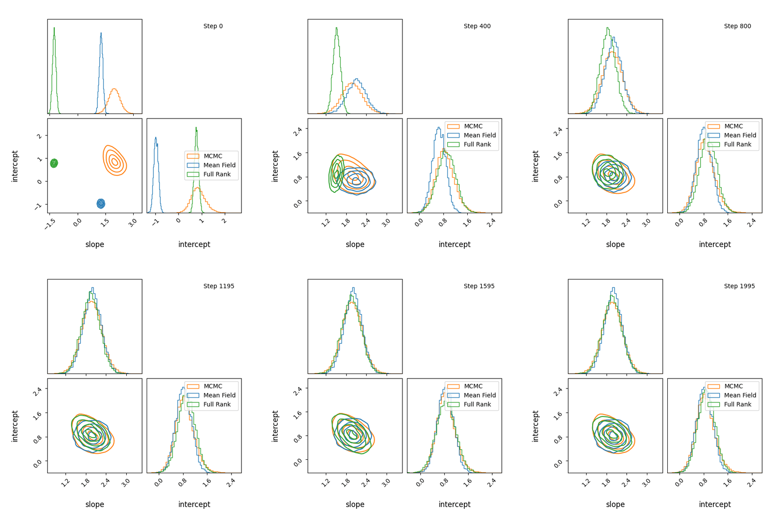
Here’s how the approximations progress and how they look! The full rank gaussian has some covariance matching the “true” posterior!

Limitations

Okay, so now we have a relatively general setup that you can use to approach posterior inference problems, but now I’m going to tell you why you (sometimes) shouldn’t use it. Of course with the above we presume that the posterior follows a gaussian distribution, which yes is a little restrictive, but the most restrictive assumption is that your posterior isn’t multi-modal.

For example, let’s have at look at a mixture model with known contributions, without order statistics, we get label switching. Let’s otherwise use the same code as above.

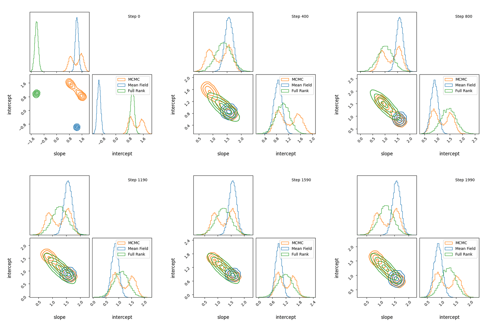
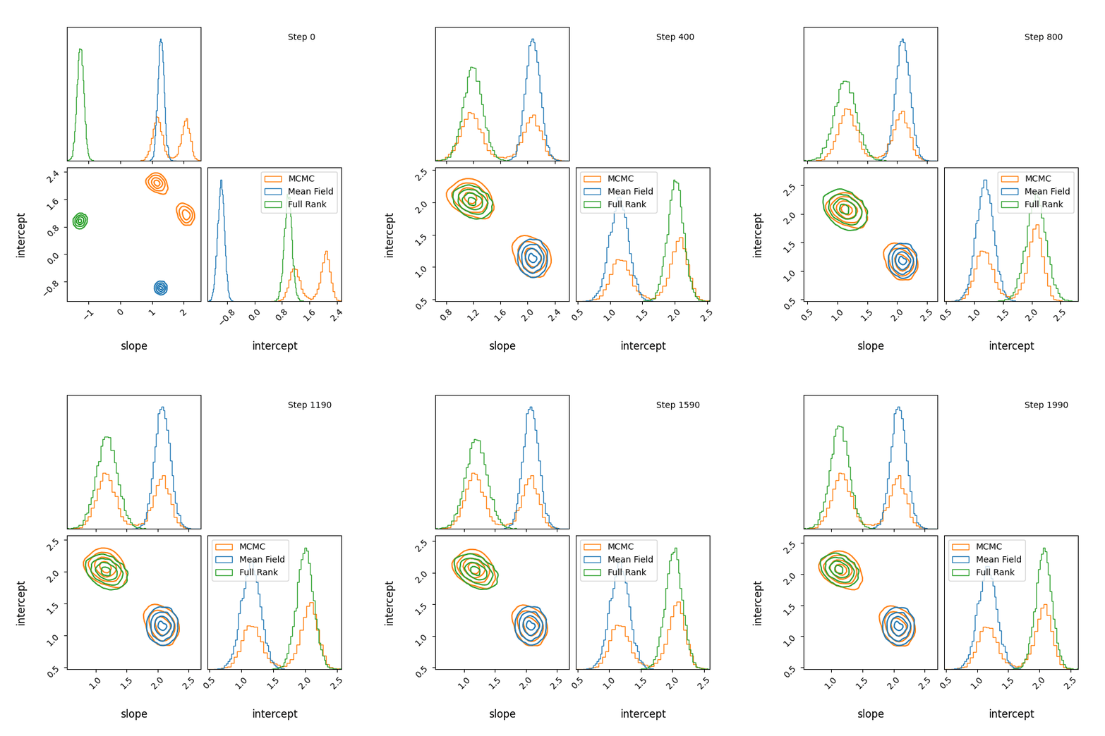
You can see that they totally miss the multi-modality (of course) but ADVI only found one of the modes but the full rank approximation tried to cover both, which only happens when the modes are nearby. If I made the slope values further apart then it’s just as bad as ADVI.

Further Reading

So now we’re aware of these relatively basic methods, I’ll leave some links for other methods that might interest you.

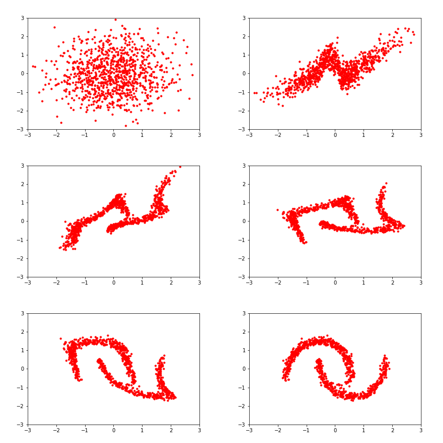
• Normalising Flows
  • A much more expressive extension to ADVI where you lean into the transformations even more (kind of)
  • You train a set of neural networks (for example) that transform some simple distribution’s samples into some arbitrary shape
  • Resources
    • (self-plug) Normalising Flows for Variational Inference (with FlowJAX)
    • Normalizing Flows: An Introduction and Review of Current Methods - Kobyzev, Prince, Brubaker
    • Variational Inference: A Review for Statisticians - Blei, Kucukelbir, McAuliffe
    • FlowJAX (python package for using normalising flows)
    • Normalizing Flows - Introduction (Part 1) - NumPyro implementation and introduction to normalising flows
    • Normalizing Flows in 100 Lines of JAX - Eric Jang

• Variational Autoencoders (VAEs)

• Generative Adversarial Networks

• Amortized Variational Inference

• Structured Variational Inference

Appendices

ADVI GIF Code

import os
import numpy as np
import matplotlib.pyplot as plt
import corner
import imageio
from jax import random
from tqdm import tqdm

# ----------- CONFIG -----------
gif_path = "advi_progress.gif"
num_frames = len(history_mf)  # assuming this is saved during training
frame_skip = 5                # plot every nth frame
sample_shape = (10000,)

# ----------- PREP ------------
frames = []
rng = random.PRNGKey(123)

# MCMC: fixed samples
samples_mcmc = np.stack([mcmc_samples['slope'], mcmc_samples['intercept']], axis=-1)

# ----------- LOOP ------------
for i in tqdm(range(0, num_frames, frame_skip)):
    # MF samples at this step
    params_mf_step = history_mf[i]  # dict with params
    posterior_mf_step = guide_mf.sample_posterior(random.split(rng)[0], params_mf_step, sample_shape=sample_shape)
    samples_mf = np.stack([posterior_mf_step['slope'], posterior_mf_step['intercept']], axis=-1)

    # FR samples at this step
    params_fr_step = history_fr[i]
    posterior_fr_step = guide_fr.sample_posterior(random.split(rng)[1], params_fr_step, sample_shape=sample_shape)
    samples_fr = np.stack([posterior_fr_step['slope'], posterior_fr_step['intercept']], axis=-1)

    # --------- PLOT ----------
    fig = plt.figure(figsize=(6, 6), dpi=100)

    # MCMC
    corner.corner(samples_mcmc, fig=fig, smooth=0.95, plot_datapoints=False, plot_density=False,
                  color="tab:orange", fill_contours=False, bins=40,
                  hist_kwargs={'density': True, 'color': 'tab:orange'},
                  labels=["slope", "intercept"], label_kwargs={"fontsize": 12})

    # Mean Field
    corner.corner(samples_mf, fig=fig, smooth=0.95, plot_datapoints=False, plot_density=False,
                  color="tab:blue", fill_contours=False, bins=40,
                  hist_kwargs={'density': True, 'color': 'tab:blue'})

    # Full Rank
    corner.corner(samples_fr, fig=fig, smooth=0.95, plot_datapoints=False, plot_density=False,
                  color="tab:green", fill_contours=False, bins=40,
                  hist_kwargs={'density': True, 'color': 'tab:green'})

    # Remove background
    fig.patch.set_facecolor('white')  # Or 'none' if using transparency
    for ax in fig.get_axes():
        ax.set_facecolor('white')
    plt.legend(["MCMC", "Mean Field", "Full Rank"])

    # Annotate frame
    ax = fig.get_axes()[1]
    ax.text(0.6, 0.9, f"Step {i}", transform=ax.transAxes)

    # Save frame
    fig.canvas.draw()
    image = np.asarray(fig.canvas.buffer_rgba())[..., :3]
    frames.append(image)
    plt.close(fig)

# --------- SAVE GIF ----------
imageio.mimsave(gif_path, frames, duration=0.3, loop=0)
print(f"Saved GIF: {gif_path}")

Separated Multi-Modal Posterior NumPyro Code

# ---------- 1. Define Mixture of Two Lines ----------
def mixture_of_lines(X, Y=None):
    # Priors
    slope1 = numpyro.sample("slope1", dist.Normal(0, 5))
    slope2 = numpyro.sample("slope2", dist.Normal(0, 5))
    # Fixed mixture weights
    w1 = true_w1
    w2 = 1.0 - true_w1

    # Compute means for each component
    mean1 = slope1 * X + true_intercept
    mean2 = slope2 * X + true_intercept

    # components1 and components2 are shape [N]
    components1 = dist.Normal(loc=mean1,scale=true_sigma).log_prob(Y,)
    components2 = dist.Normal(loc=mean2,scale=true_sigma).log_prob(Y,)


    log_mixture_likelihood = jnp.logaddexp(jnp.log(w1)+components1, jnp.log(w2)+components2).sum()

    # expose log-like to NumPyro
    numpyro.factor("loglike", log_mixture_likelihood)




# ---------- 2. Run SVI ----------
def run_svi(guide_class, rng_key, lr=0.01, decay_rate=0.75, end_value=1e-4, schedule='exponential'):
    guide = guide_class(mixture_of_lines)
    total_steps = 2000

    # Learning rate schedule
    if schedule == 'exponential':
        schedule_fn = optax.exponential_decay(
            init_value=lr,
            transition_steps=100,
            decay_rate=decay_rate,
            staircase=True
        )
    else:
        schedule_fn = optax.linear_schedule(
            init_value=lr,
            end_value=end_value,
            transition_steps=total_steps
        )

    optimizer = optax.adam(schedule_fn)
    svi = SVI(mixture_of_lines, guide, optimizer, loss=Trace_ELBO())

    svi_state = svi.init(rng_key, X, Y)

    losses = []
    history = []  # << Store parameter snapshots here

    for i in range(total_steps):
        svi_state, loss = svi.update(svi_state, X, Y)
        losses.append(loss)

        # Save parameters for this step
        params = svi.get_params(svi_state)
        history.append(params)

        if i % 100 == 0:
            print(f"Iter {i}: loss = {loss:.2f}")

    final_params = svi.get_params(svi_state)
    return guide, final_params, losses, history




# ---------- 3. Mean Field Guide ----------
print("Running Mean Field ADVI")
key1, key2 = random.split(rng_key)
guide_mf, params_mf, losses_mf, history_mf = run_svi(AutoDiagonalNormal, key1, lr=0.01, decay_rate=0.85)

# ---------- 4. Full Rank Guide ----------
print("Running Full Rank ADVI")
guide_fr, params_fr, loss_fr, history_fr = run_svi(AutoMultivariateNormal, key2, lr=0.1, end_value = 5e-4, schedule='linear')