Normalising Flows for Variational Inference (with FlowJAX)

In this post, I’ll attempt to give an introduction to normalising flows from the perspective of variational inference.

Below are the resources I’m using as references for this post. Feel free to explore them directly if you want more information or if my explanations don’t quite click for you:

• Variational Inference with Normalizing Flows — Rezende, 2015
  • This is the reference I connected with the most when learning general variational inference. Highly recommended.
• Normalizing Flows: An Introduction and Review of Current Methods — Kobyzev, 2020
  • Focused specifically on normalising flows. I found it a bit confusing at times due to frequent switching of variable names, but the core ideas are clearly presented.
• “Normalizing Flows” by Didrik Nielsen — Probabilistic AI School
• “Density estimation using Real NVP” — Dinh, 2016
• “Masked Autoregressive Flow for Density Estimation” — Papamakarios, 2018

Table of Contents

• Variational Inference
• Normalising Flows
• Normalising Flows with Neural Network-Mediated Transforms
• Examples
  • Example: 2D with 4D Posterior
  • Example: Hierarchical Bayesian Model Analysis with 25D Posterior
• Some Annoying Things…

Variational Inference

A common goal in Bayesian analysis is to develop a posterior distribution for inference:

Bayesian inference methods typically approach this by sampling from the posterior using algorithms like MCMC or nested sampling. These methods rely on the product of the likelihood \(p(x \mid z)\) and the prior \(p(z)\):

The goal is to produce representative samples of the posterior distribution. MCMC and nested samplers are theoretically exact in their limits — if you run MCMC indefinitely or increase the number of live points to infinity in nested sampling, you’ll converge to the true posterior (or at least close enough that the difference doesn’t matter in practice).

Variational inference, by contrast, trades this potential for exactness in favour of approximating the posterior with a simpler distribution from a tractable family.

You define a family of candidate distributions, denoted \(\mathcal{Q}\), and find the member of that family which is closest (in KL divergence) to the true posterior. The true posterior may or may not lie within \(\mathcal{Q}\), but we optimise for the best approximation available within that set.

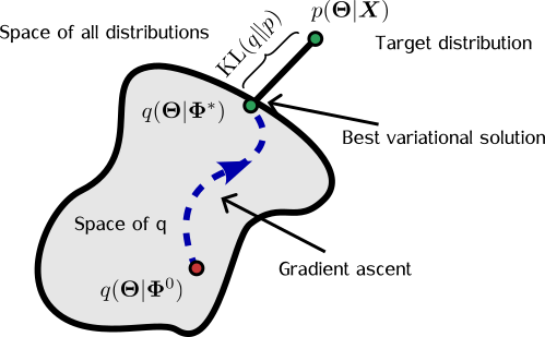
You might prefer methods that guarantee convergence to the exact posterior, but variational inference advocates would argue that we never truly reach exactness in practice anyway, so we might as well adopt an approximation method that’s efficient and easier to work with.

I generally agree with this view, but there are a few caveats to keep in mind throughout this post:

• The function family \(\mathcal{Q}\) may not include anything that approximates the true posterior particularly well.
  • For example, a Laplace approximation may struggle with a posterior involving a mixture model, where variables could be better described by an uninformative Dirichlet — something a Gaussian would approximate poorly.
• As far as I know, there aren’t great tools to analyse convergence of variational inference the way we can with MCMC (e.g., using autocorrelation) or nested sampling (e.g., using \(\text{dlogz}\)).
  • That said, in my experiments, once the ELBO loss flattens out, further training usually doesn’t improve results much — and this has generally been “good enough.”

Still, one of the strongest advantages I’ve found with variational methods is that they give you a parametric form for your posterior, which is extremely useful. More importantly, they convert the posterior estimation problem from one of sampling to one of optimisation. This makes the problem more tractable and opens the door to using modern optimisation techniques to speed up your analysis.

The Formal Goal of Variational Inference

Let’s say we approximate the posterior with a distribution \(q_\Phi(z) \in \mathcal{Q}\), where \(\Phi\) are the parameters controlling its shape. Then, the formal objective of variational inference is:

That is: find the parameter set \(\Phi^*\) such that \(q_{\Phi^*}(z)\) is the closest element in \(\mathcal{Q}\) to \(\pi(z \mid x)\), in terms of KL divergence. In this setup, the densities are normalised with respect to \(z\), not \(\Phi\). The problem of sampling from a posterior becomes one of minimising a loss function.

We can also expand the KL divergence:

Rearranging:

Since the KL divergence is non-negative, the ELBO is indeed a lower bound on the log evidence \(\log \mathcal{L}(x)\). Conveniently, ELBO only involves the joint distribution \(p(z, x)\) and the approximate posterior \(q(z)\), not the true posterior itself. This means we can maximise the ELBO using standard likelihood-prior products to identify the optimal approximate posterior \(q_{\Phi^*}(z)\).

Normalising Flows

Normalising flows, in a nutshell, are a way of constructing an approximate posterior in variational inference by transforming simple probability distributions into more complex ones through a series of invertible, differentiable mappings.

Suppose we have a random variable \(Y\) with a known, tractable probability distribution \(p_Y\), and we define a transformation such that \(Z = g(Y)\) or equivalently \(Y = f(Z)\). Then the probability density of \(Z\) is:

where \(\mathbf{Df}(z) = \frac{\partial f}{\partial z}\) is the Jacobian of \(f\) with respect to \(z\), and similarly \(\mathbf{Dg}(y) = \frac{\partial g}{\partial y}\) is the Jacobian of \(g\) with respect to \(y\). In this context, \(p_Z(z)\) is sometimes referred to as the pushforward of \(p_Y\) by the function \(g\), denoted \(g_* p_Y\).

The term normalising in “normalising flows” comes from the inverse mapping \(f\), which transforms the (possibly complex) variable \(Z\) into the simpler \(Y\). Essentially, this “normalises” the data to a distribution we know how to work with, such as a standard Gaussian.

So far, this setup involves just a single transformation \(g\), but because invertible functions can be composed, we can create a chain of such transformations:

with corresponding inverse:

The determinant of the total Jacobian of \(f\) can then be expressed as the product of the Jacobians of each component:

where each intermediate variable \(s_i\) is defined as:

with \(s_N = z\). This stacking allows us to combine relatively simple, expressive transformations into highly flexible and powerful composite mappings capable of modelling very complex posteriors.

An intuitive demonstration of this idea is shown below, from a GIF by Eric Jang in his tutorial on normalising flows, which focuses on how to implement flows using JAX:

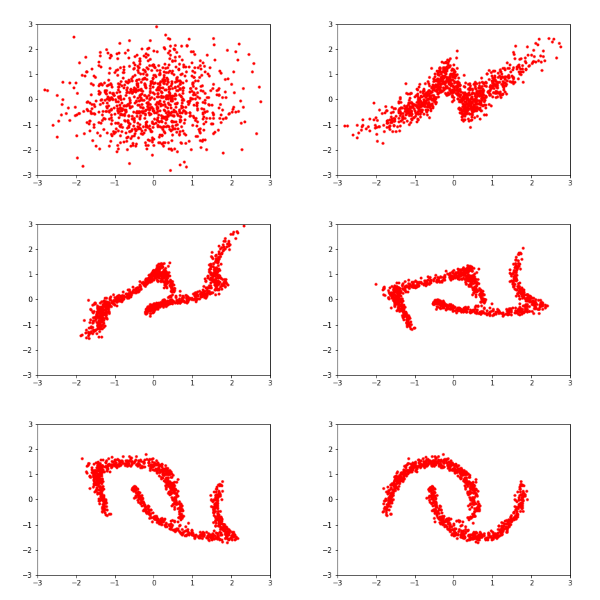
Back to the math: since we typically prefer working in log-space for numerical stability, we can write the log-likelihood of a set of samples \(\mathcal{Z}\) from the transformed distribution as:

Here, \(\theta\) denotes the parameters controlling the transformations, and \(\phi\) parameterises the base distribution \(p_Y\). Together, these represent the full parameter set \(\Phi = \{\theta, \phi\}\).

During training, the main parameters to optimise are those of the transformations \(\theta\), and of the base distribution \(\phi\), in order to maximise the ELBO. A useful identity allows us to compute expectations with respect to \(p_Z\) in terms of the base distribution:

for any function \(h\), treating \(\phi\) as constant (since any dependence on it can typically be rolled into \(\theta\) anyway). This identity is useful for calculating gradients during optimisation: instead of needing to differentiate through a sampling distribution, we can use this reparameterisation trick to move the dependence on \(\theta\) inside the integrand. That makes computing gradients with respect to \(\theta\) far more straightforward.

The Process

In practical terms, the general process for using normalising flows in variational inference looks like this:

1. Sample \(z\) from the current approximation \(q(z \mid \theta)\)
2. Compute the probability of this sample under both \(q(z \mid \theta)\) and the joint \(\mathcal{L}(x \mid z) \pi(z)\)
3. Calculate the Jacobian and its log determinant
4. Update the transformation parameters using gradient-based optimisation

Examples of Flow Methods

Your next question should be then, well what are the transformations?? What should I specifically make \(g\)/\(f\)?? Well the class of functions that you wish to consider basically dictates the overall approach that you want to take. I’ll show some examples of different methods building up to the ultimate goal of this post which is variational inference with normalising flows with neural network assisted transformations.

Linear Flows

Linear flows are normalising flows that utilise transformations of the form,

where \(A \in \mathbb{R}^{D\times D}\) and \(b_i\in \mathbb{R}^D\) and \(D\) is the dimensionality of \(z\). These types of transformations are relatively restricted in the complexity of posteriors they can express, but are simpler to implement compared to other methods while still being able to capture many less pathological distributions. The determinant of the jacobian of the transformation is just the determinant of \(A\) and the inverse transformation just \(A^{-1}\) (and the total transformation just the product of all of these), but both operations can be expensive in high dimensions with complexities of \(\mathcal{O}(D^3)\). However, we can restrict the form of \(A\) to increase the efficiency of these operations.

And then you can layer these transformations (letting \(g=g_i\) above) to create a more flexible model.

Diagonal-Linear Flows

If \(A\) is a diagonal matrix, the inverse is just the reciprocal of the diagonal elements and the determinant is the product of the elements on the diagonal which are both \(\mathcal{O}(D)\). However, this transformation turns into an element-wise transformation which makes it impossible to capture the correlation between variables.

Triangular-Linear Flows

If we make \(A\) a lower or upper triangular matrix then we can theoretically capture the correlations between variables because multiple variables from the base distribution can mix, but additionally the matrix determinant is still just the product of the diagonal, and matrix inversion is \(\mathcal{O}(D^2)\) instead of \(\mathcal{O}(D^3)\) for general matrix inversion.

Coupling Flows

Coupling flows are set up such that the transforms are conditioned on other values of the variables in posterior of interest. i.e. If you have a D-dimensional posterior still denoted with \(\vec{z} = \{z_1, z_2, ..., z_d, z_{d+1}, ..., z_D\}\) and \(y\) and \(x\) follow this same dimensionality. A coupling flow in this scheme is constructed as a hybrid function, remembering that \(\vec{s}\) is our fill in “intermediary variable” between \(y\) and \(z\), such that,

In essence, you leave some parts of your intermediary variable alone, \(s_{d+1:D}\) , and then transform the rest, \(s_{1:d}\), based on some coupling function \(h\) with parameters based on some conditioner \(\Theta\) that are dependent on the part of the variable we leave alone, \(x_{d+1:D}\). The assumption being that you would then apply some permutation function inbetween subsequent layers so that you apply a transformation to every value in \(y\) (so you wouldn’t really have \(z\) on the left above but the next stage of the intermediary variable \(s\) but that’d be confusing).

This approach is nice as you get a lot of expressiveness out of it (depending on what you choose for \(h\)) while gives you a block triangular matrix with the blocks being the identity matrix and \(Dh\) (which is just \(d\times D-d\) as opposed to \(D\times D\)). The method by which you partition it is then up to you, but it’s common to either split it in half or do some alternating pixels if you are looking at image data.

Additionally, \(\Theta\) can be as complex as you like and is often represented using a neural network (but not the goal of this post).

The inverse then looks like (presuming that the inverse, \(h^{-1}\), exists),

Autoregressive Flows

General autoregressive models outside of just normalising flows describe the probability of a given event or variable as some sort of function on previous events/variables. i.e. If I have a variable \(x=(x_1, x_2, ..., x_d)\) then an autoregressive model might describe the probability as¹,

This has a nice extensions to what we’re doing with our intermediate variables \(s_i\).

We generate the samples as

where \(\Theta_1\) is a constant. This is extremely similar to what we saw in the coupling flows except instead of our transformation is blocks of \(\vec{s}\) being transformed into blocks of \(\vec{s}\) they are now of blocks of \(\vec{s}\) being transformed into specific values of \(\vec{s}\), \(s_i\). The functions also retain the same terminology. So the determinant here is given by²,

The difficulty for this style of flow is the calculation of the inverse that has to be found using recursion (icky) and inherently sequential as,

Despite this drawback autoregressive models have been shown to have an extreme level of flexibility at capturing complex distributions (e.g. Papamakarios, 2017). And additionally, there is a related architecture called “inverse autoregressive flows” where \(z_i = h(s_i;\theta(z_{1:i-1}))\) that has the inverse problem that the forward direction is hard to compute but the inverse is simple, i.e. that it is quicker to sample and is thus better suited to methods within variational inference that require lots of sampling.

Examples of coupling functions

Well after all that it may seem like I’ve kicked the can down the road as the question was “what functions should I use for my transformations” and now I’ve left the answer open because now you’re likely asking “well what should I use for my coupling functions!”. Well for now I would just look at the titles as they’re pretty self-explanatory, and I want to finish this post.

Affine Coupling Functions

Cubic Splines

Rational Quadratic Splines

Notable mentions of approaches that I did not cover

• Sequential Neural Posterior estimation (see e.g. Automatic Posterior Transformation for Likelihood-Free Inference or On Contrastive Learning for Likelihood-free Inference)
  • A method where you skip the use of priors and likelihoods and instead estimate the posterior using simulations based on the parameters of interest
• Unconditional density estmation
  • If you have a samples from the distribution directly and wish to construct a parametric form
• RealNVP
  • A very successful approach to normalising flows algorithm
• Continuous Flows
  • Not even sure how this one works but it looks neat
• Many others, I’d highly recommend looking at all the resources I’ve linked to above for more info.

Normalising Flows with neural network mediated transforms (Neural Autoregressive Flows)

Thanks for sticking around this far (and welcome, if you skipped most of the post and are just here for the conclusion). The final cherry on top is that, although normalising flows are ultimately an optimisation problem, we can leverage recent advancements in machine learning—particularly neural networks—to improve their flexibility and expressiveness.

There isn’t much new theory here: you’re simply replacing the conditioning mechanisms in your coupling functions (i.e., the \(\Theta\)’s from earlier) with neural networks. One might ask: why not just use neural networks as the transformations themselves?

While that sounds reasonable in theory, in practice it poses challenges. General neural network transformations tend to be dense, making the resulting mappings difficult or impossible to invert analytically or efficiently. Many common flow architectures—like coupling flows or autoregressive flows—are specifically designed to ensure tractable Jacobians and invertibility. Letting neural networks control the parameters of these structured flows maintains these guarantees while still benefiting from neural nets’ flexibility.

As before, I highly recommend Eric Jang’s tutorial if you’re interested in coding up a normalising flow yourself using JAX. Personally, though, I prefer to avoid the inevitable debugging headaches and use an off-the-shelf solution whenever possible.

In my case, I’ve had good experiences with the FlowJAX Python package, and also found solid support in PyTorch and TensorFlow ecosystems.

In the next section, I’ll walk through a few examples of how to use FlowJAX for variational inference and compare it with traditional samplers.

Examples Analyses

Example: Simple 4D Latent Model – Normalising Flows and Nested Sampling Comparison

We’ll start with a relatively simple example: data in 2D generated from a mixture of two linear models, each with its own intrinsic scatter (i.e., model-dependent noise). Specifically:

We assume the first model has a fixed intercept (i.e., \(c_1 = 0\)) to reduce identifiability issues. The parameters to infer are \(m_1\), \(m_2\), \(c_2\), and one mixture fraction (since \(w_2 = 1 - w_1\)). So, we have 4 independent variables total.

Below are two plots showing the simulated data: one with colours indicating the source model, and one showing the raw observed scatter.

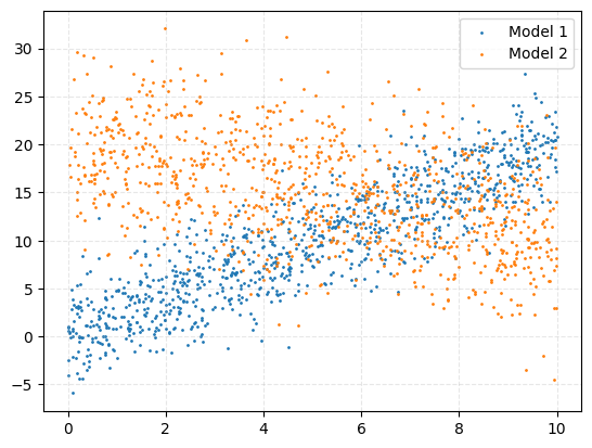
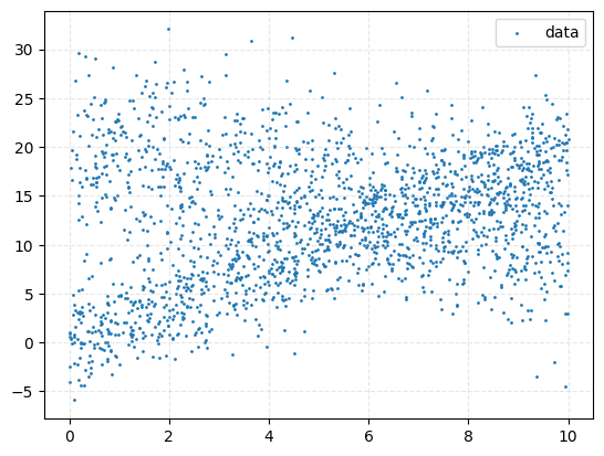
Now, we’ll apply both a normalising flow and nested sampling to this problem and compare the results. The likelihood for a given point \((x_i, y_i)\) is:

We assume uniform priors on \(m_1\), \(m_2\), and \(c_2\), and an uninformative Dirichlet prior on the mixture fractions (which, for two components, is just a uniform prior over [0, 1]).

After running nested sampling, we get the following posterior distribution:

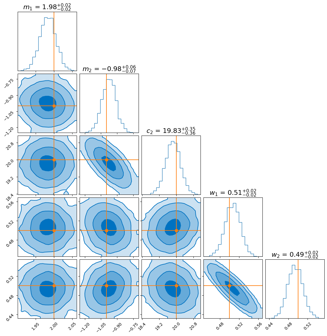
Now let’s try the same with JAX and FlowJAX.

We define our log-likelihood and prior as follows:

def jax_event_loglikelihood(yval, xval, mval, sigmaval, cval):
    return jax.scipy.stats.norm.logpdf(yval, loc=mval * xval + cval, scale=sigmaval)

def jax_total_loglikelihood(theta, yvals, xvals):
    m1val, m2val, c2val, w1, w2 = theta
    w2 = 1 - w1  # ensure constraint
    return jnp.sum(jax.scipy.special.logsumexp(
        jnp.array([
            jnp.log(w1) + jax_event_loglikelihood(yvals, xvals, m1val, sigmaval=model_1_config['s'], cval=model_1_config['c']),
            jnp.log(w2) + jax_event_loglikelihood(yvals, xvals, m2val, sigmaval=model_2_config['s'], cval=c2val),
        ]),
        axis=0
    ))

def jax_logprior(theta):
    m1val, m2val, c2val, w1, w2 = theta
    m1_logprob = jax.scipy.stats.uniform.logpdf(m1val, loc=-10, scale=20)
    m2_logprob = jax.scipy.stats.uniform.logpdf(m2val, loc=-10, scale=20)
    c2_logprob = jax.scipy.stats.uniform.logpdf(c2val, loc=-50, scale=100)
    mixture_logprob = jax.scipy.stats.dirichlet.logpdf(jnp.array([w1, w2]), alpha=jnp.array([1, 1]))
    mixture_logprob = jnp.where(jnp.isnan(mixture_logprob), -jnp.inf, mixture_logprob)
    return m1_logprob + m2_logprob + c2_logprob + mixture_logprob

def unregulariser(theta_reg):
    m1val_reg, m2val_reg, c2val_reg, w1val_reg = theta_reg
    m1val = m1val_reg * 20 - 10
    m2val = m2val_reg * 20 - 10
    c2val = c2val_reg * 100 - 50
    w1val = w1val_reg
    w2val = 1 - w1val
    return (m1val, m2val, c2val, w1val, w2val)

def unnormalised_posterior(theta):
    theta = unregulariser(theta)
    return jax_logprior(theta) + jax_total_loglikelihood(theta, yvals=y_vals, xvals=x_vals)

From here, we can just drop this into our favourite inference engine—like FlowJAX:

from flowjax.bijections import Affine, RationalQuadraticSpline
from flowjax.distributions import Normal
from flowjax.flows import masked_autoregressive_flow
from flowjax.train import fit_to_key_based_loss
from flowjax.train.losses import ElboLoss
import jax.random as jr

key = jr.key(0)
loss = ElboLoss(unnormalised_posterior, num_samples=500)
key, flow_key, train_key, sample_key = jr.split(key, 4)

flow = masked_autoregressive_flow(
    flow_key,
    base_dist=Normal(loc=jnp.array([0.5, 0.5, 0.5, 0.5]), scale=jnp.array([0.01, 0.01, 0.01, 0.01])),
    transformer=RationalQuadraticSpline(knots=4, interval=(0, 1)),
    invert=False,
)

flow, losses1 = fit_to_key_based_loss(train_key, flow, loss_fn=loss, learning_rate=1e-2, steps=100)
flow, losses2 = fit_to_key_based_loss(train_key, flow, loss_fn=loss, learning_rate=1e-3, steps=200)

This gives us a nice ELBO loss curve. Note that the ELBO is a lower bound on the evidence, so it’s not expected to go to zero — here, I offset the curve by its minimum value for display purposes:

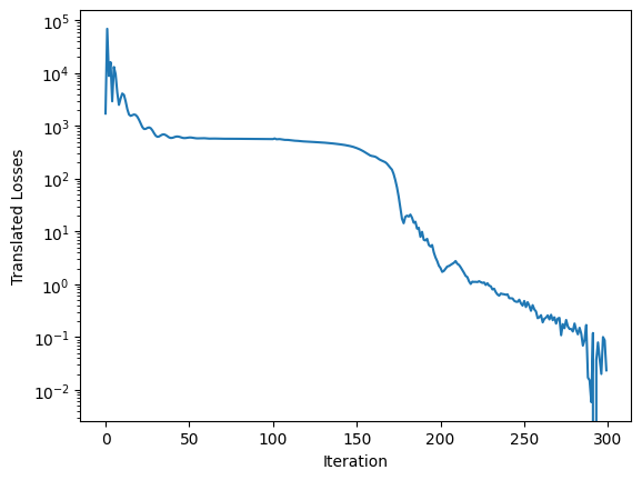
And finally, here’s the approximate posterior obtained from the normalising flow:

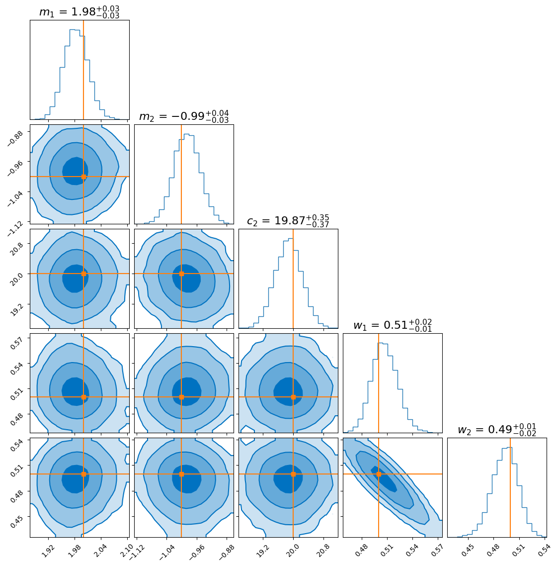
To compare, we overlay the flow-derived posterior with the one obtained from nested sampling:

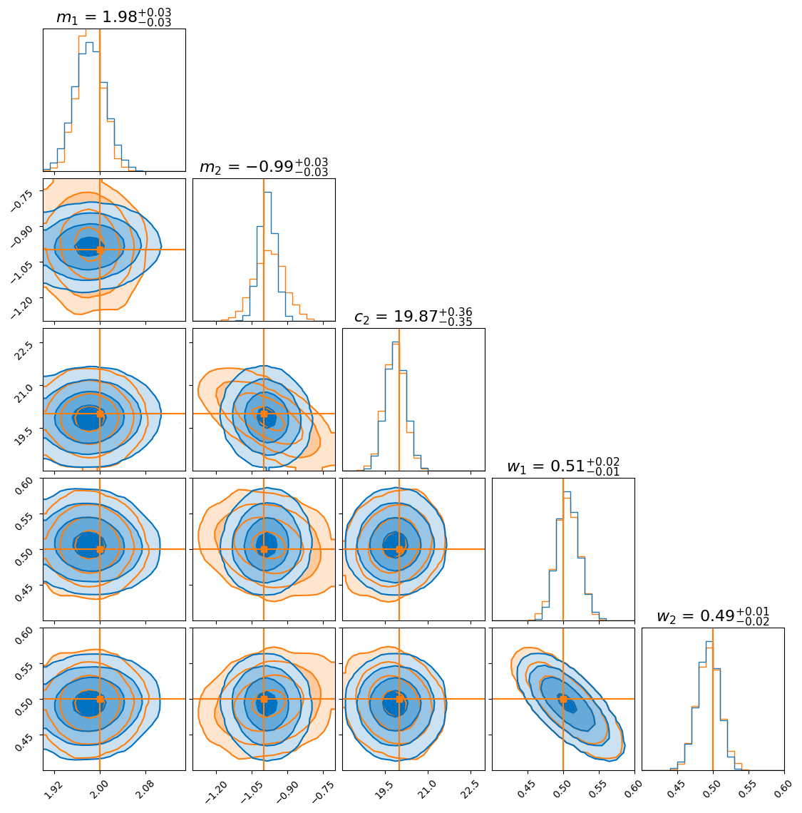
As you can see, the distributions agree closely for most parameters. However, the flow seems to produce a more sharply peaked distribution for the gradient of the second model (\(m_2\)). This doesn’t necessarily mean the flow is “better”—in fact, it likely underestimates the uncertainty, which is a known tendency in variational inference.

Example: Hierarchical Bayesian Model Analysis

The only reason that you should be interested in normalising flows should be either some benefit of getting a parametric representation out of your analysis, the dimensionality of your problem is high (and you don’t have or can’t be bothered finding yourself gradient data) or you’ve got some pathological posterior that other samplers are having trouble with. For this next example I was hoping to show this to you but could only get as far as 26 dimensions for reasons that I will explain after this example.

For this example we’re going to look at pseudo-particle tracking data where you have a three straight lines with gaussian intrinsic scatter going through \(x\), \(y\), \(z\) with parametric representations based on time \(t\) which is sampled uniformly from \(-20\) to \(20\) and a “deposited energy” variable \(E\) that follows an exponential relationship with \(t\) (in hopes of reproducing the general behaviour of a particle exponentially losing energy over time). This data is shown in the first row of GIFs. We then add gaussian noise to the spatial data and log-normal noise to the energy data (independent of time and each other for simplicity) with some background noise that is just uniform in space and log-uniform in energy (again independent of time).

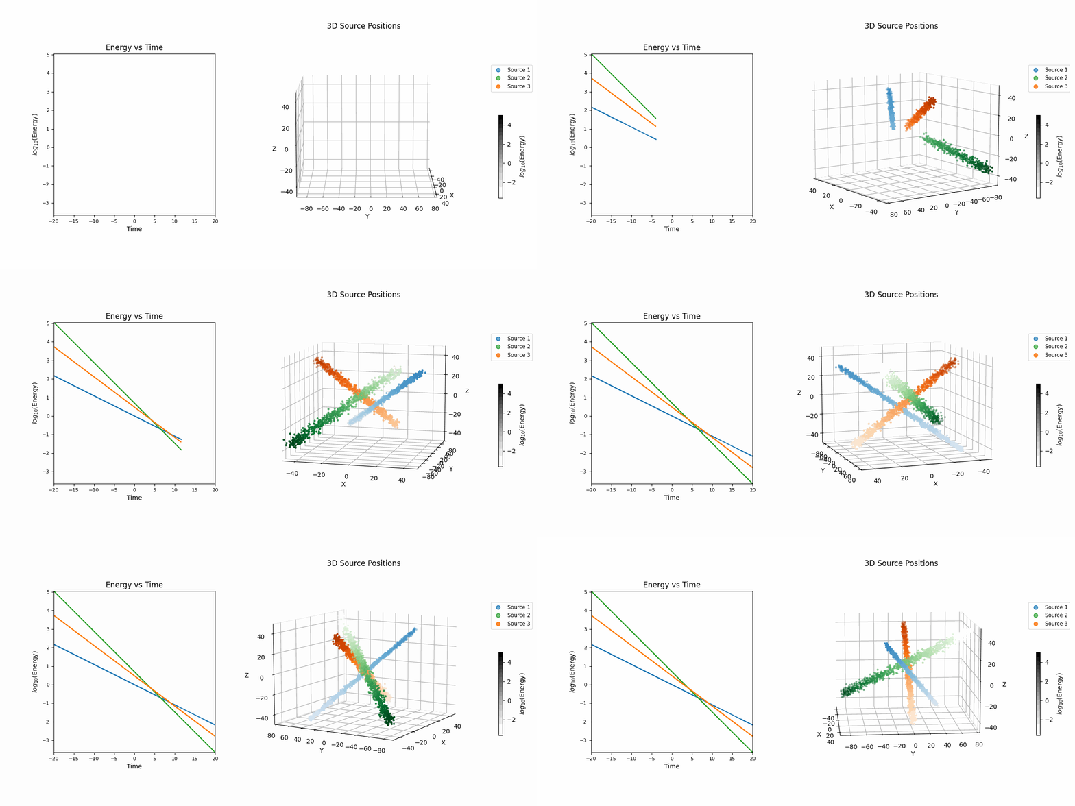
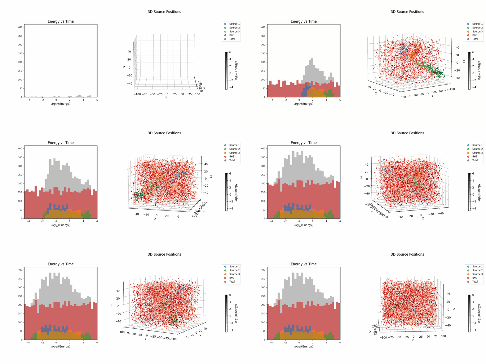
In essence, for the true values,

then we add noise to mimic a detector,

So we do the same old song and dance of making a prior (which is made up of either normal or log-normal distributions roughly about where the true values are to I’m less likely to run into instability issues) and likelihood with the addition of this handy class to handle any constrained variables,

import jax
import jax.numpy as jnp
from jax import nn
from typing import ClassVar
from flowjax.bijections import AbstractBijection, Affine
from collections.abc import Callable
from functools import partial
from typing import ClassVar

import jax.numpy as jnp
from jax.nn import softplus
from jax.scipy.linalg import solve_triangular
from jaxtyping import Array, ArrayLike, Shaped
from paramax import AbstractUnwrappable, Parameterize, unwrap
from paramax.utils import inv_softplus

from flowjax.bijections.bijection import AbstractBijection
from flowjax.utils import arraylike_to_array
from jax.scipy.special import logit  # Import logit


class SigmoidAffine(AbstractBijection):
    r"""Sigmoid and affine transformation combined: 
    First, applies Sigmoid(x) and then applies affine transformation y = a * x + b.

    Args:
        loc: Location parameter for the affine transformation. Defaults to 0.
        scale: Scale parameter for the affine transformation. Defaults to 1.
    """

    shape: tuple[int, ...]
    cond_shape: ClassVar[None] = None
    loc: jax.Array
    scale: jax.Array

    def __init__(
        self,
        loc: ArrayLike = 0,
        scale: ArrayLike = 1,
    ):
        # Convert loc and scale to arrays using arraylike_to_array utility
        self.loc = arraylike_to_array(loc, dtype=float)
        self.scale = arraylike_to_array(scale, dtype=float)

        # Ensure loc and scale are broadcastable
        self.loc, self.scale = jnp.broadcast_arrays(self.loc, self.scale)
        self.shape = self.scale.shape

    def transform_and_log_det(self, x, condition=None):
        # Apply Sigmoid first
        sigmoid_x = nn.sigmoid(x)
        # Apply affine transformation
        y = sigmoid_x * self.scale + self.loc
        log_det_affine = jnp.sum(jnp.log(jnp.abs(self.scale)))

        # Log determinant from the sigmoid transformation
        log_det_sigmoid = jnp.sum(nn.log_sigmoid(x) + nn.log_sigmoid(-x))

        # Total log determinant is the sum of both log determinants
        log_det = log_det_sigmoid + log_det_affine
        return y, log_det

    def inverse_and_log_det(self, y, condition=None):
        # Apply inverse of affine transformation
        affine_inv_x = (y - self.loc) / self.scale
        log_det_affine = -jnp.sum(jnp.log(jnp.abs(self.scale)))

        # Apply inverse of Sigmoid (logit function)
        x = logit(affine_inv_x)

        # Log determinant from the sigmoid inverse transformation
        log_det_sigmoid = -jnp.sum(nn.log_sigmoid(x) + nn.log_sigmoid(-x))

        # Total log determinant is the sum of both log determinants
        log_det = log_det_sigmoid + log_det_affine
        return x, log_det

We can then set up the flow as the following,

from flowjax.bijections import Affine, Sigmoid, Identity, RationalQuadraticSpline
from flowjax.distributions import Normal, StudentT, Transformed
from flowjax.flows import masked_autoregressive_flow, triangular_spline_flow, block_neural_autoregressive_flow
from flowjax.train import fit_to_key_based_loss
from flowjax.train.losses import ElboLoss
import jax.random as jr
from paramax import non_trainable

key = jr.key(0)

def create_bijections():
    # Bijections for each parameter to enforce bounds. But most follow a normal distribution instead of uniform where bounds are required, 
        # so identity is used
def create_bijections():
    # Bijections for each parameter to enforce bounds
    bijections = []

    ## Model 1 Stuff
    # as
    bijections.append(Identity())
    bijections.append(Identity())
    bijections.append(Identity())
    # bs
    bijections.append(Identity())
    bijections.append(Identity())
    # es
    bijections.append(Identity())
    bijections.append(Identity())


    ## Model 2 Stuff
    # as
    bijections.append(Identity())
    bijections.append(Identity())
    bijections.append(Identity())
    # bs
    bijections.append(Identity())
    bijections.append(Identity())
    # es
    bijections.append(Identity())
    bijections.append(Identity())

    ## Model 3 Stuff
    # as
    bijections.append(Identity())
    bijections.append(Identity())
    bijections.append(Identity())
    # bs
    bijections.append(Identity())
    bijections.append(Identity())
    # es
    bijections.append(Identity())
    bijections.append(Identity())




    # For sigma_t (log-transformed, bounded between logt_loc and logt_loc + logt_scale)
    bijections.append(Identity())

    # For sigma_e (log-transformed, bounded between logsigma_e_loc and logsigma_e_loc + logsigma_e_scale)
    bijections.append(Identity())
    # For w1reg (bounded between 0 and 1, use Sigmoid to constrain it)
    bijections.append(SigmoidAffine(loc=0, scale=1))
    # For w2reg (bounded between 0 and , use Sigmoid to constrain it)
    bijections.append(SigmoidAffine(loc=0, scale=1))
    # For w3reg (bounded between 0 and , use Sigmoid to constrain it)
    bijections.append(SigmoidAffine(loc=0, scale=1))

    bijections = bij.Stack(bijections)

    return bijections




loss = ElboLoss(unnormalised_posterior, num_samples=500, stick_the_landing=True)


key, flow_key, train_key, sample_key = jr.split(key, 4)
unbounded_flow = triangular_spline_flow(
    key=flow_key,
    base_dist=Normal(loc=0.*jnp.array(list((true_vals))), 
                    scale=0.1*jnp.ones(len((true_vals)))), 
    knots=4,
    tanh_max_val=3.0,
    invert=False,
    init=None,
    flow_layers=6,
)

flow = Transformed(
    unbounded_flow,
    non_trainable(create_bijections()) # Ensure constraint not trained!
)

schedule = [(1e-2, 50),(4e-3, 50),(1e-3, 50),]  
total_losses = []
for learning_rate, steps in schedule:
    train_key, subkey = jr.split(train_key)

        # Train the flow variationally
    flow, losses = fit_to_key_based_loss(
        train_key, flow, loss_fn=loss, learning_rate=learning_rate, steps=steps,
    )
    total_losses.extend(losses)

This gave me the following loss curve. Anecdotally, I’ve found that if the loss curve follows this kind of decaying sinusoidal looking shape that the posterior flow samples are of better quality. I imagine this is because it’s found the correct minimum and is bouncing back and forth across the “well” towards the proper solution.

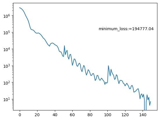
And posterior.

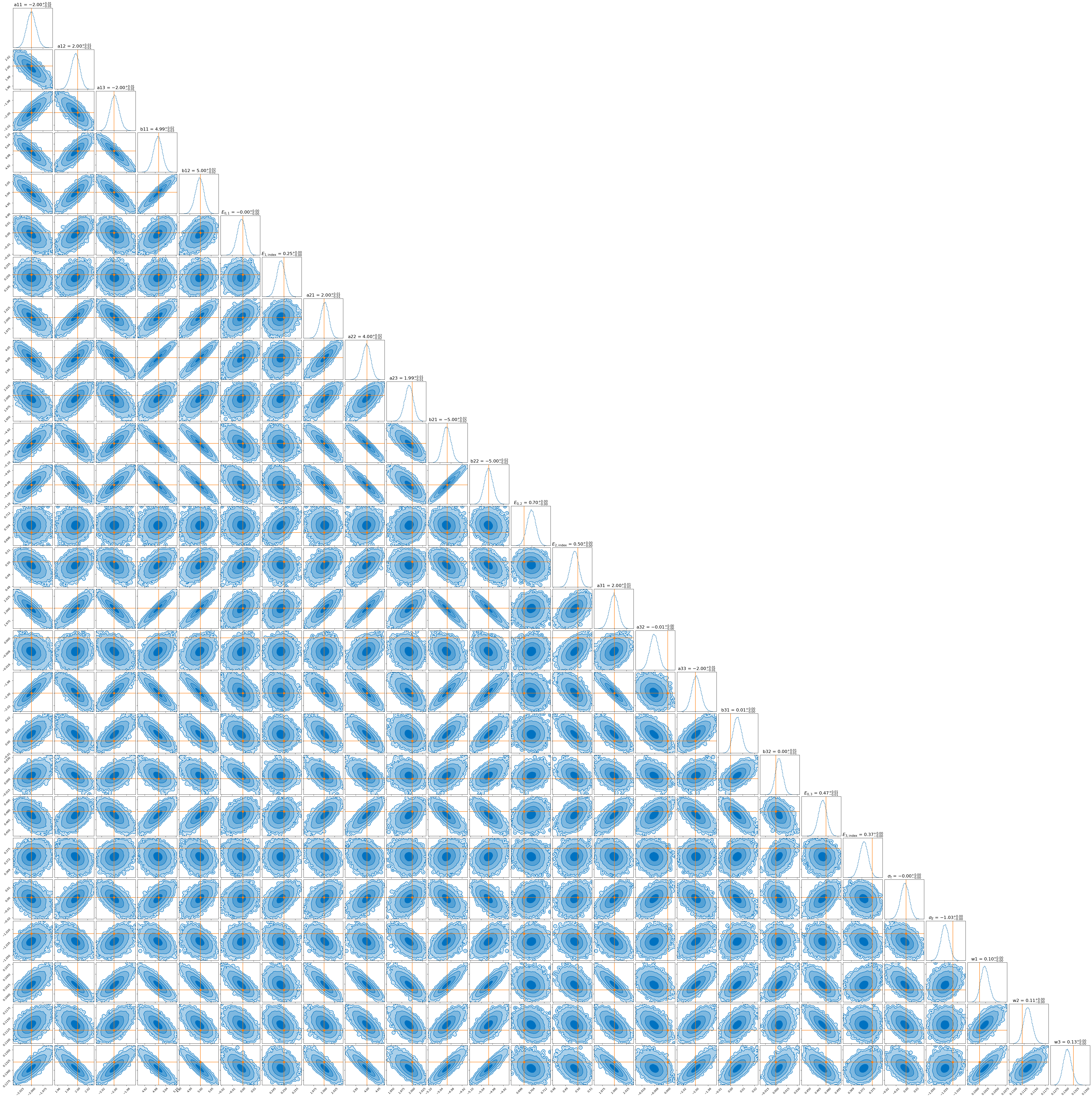
Due to needing the results to be stable for this dimensionality this run took significantly longer than the first. The normalising flow for the first example took ~30 seconds to train, while this one took ~25 minutes (although the large time for the second is likely due to my relative inexperience with flows). But hey, that’s still relatively quick for the \(10^4\) datapoints that this uses and now we have a parametric representation of our posterior that we can sample really easily and quickly.

Some Annoying Things About Normalising Flows

Despite what the benefits that I’ve tried to get across with all of the above, there are still quite a few aspects of normalising flows that are finicky enough that, personally, would mean that I wouldn’t recommend using normalising flows to the general statistician that I will highlight (mostly again) here.

1. Optimisation Instability. Despite the “speed” benefits of optimisation, due to the large number of parameters being investigated among other things, gradients are prone to explode and produce major instabilities during fitting. I’ve referenced a couple approaches to get around some of these problems below but I’ve found that at least one of them still leaves things being finicky (and the other ones I haven’t implemented yet…), and now with the stability measures, not that fast.
2. Convergence. Because this is essentially optimisation like I talk about above the only “convergence” metric is whether you think the loss curve has plateaued and because the flow is just moving around some “nice” distribution to begin with the results can still look “nice” even if it’s converged on some bogus area of the parameter space bar the following point.
3. “Is that the posterior, or some weird artefact from the transformations?” I will quite often get a posterior out from a normalising flow with a variable with a strange skew or extension in the posterior, but it is hard to tell whether this comes from the posterior actually having that shape and the flow just allows the freedom to sample enough to see this properly or whether it’s some artefact of the transformations that the normalising flow has found and left in there.
4. It’s just plain ol’ finicky. In my experience, using normalising flows has been a kind of mix of optimisation issues, general machine-learning bugs, alongside a bloody sampler. I think I solve one thing or then another problem pops up (seemingly purely out of mechanical spite). But even worse, is that I fix something that is obviously wrong, and that makes the flow stop working. For the above examples it would have been much much much quicker to use standard methods like HMC or nested sampling rather than flows (possibly out of experience, but the flows really seemed like an uphill battle).

Additionally, I have only read this as I haven’t had the need to look at discrete distributions in my posterior (and can’t be bothered making synthetic data for yet). According to Kobyzev, 2020, describing discrete distributions are an open problem.

Here are some references that include discussions on issues involving normalising flows (and in some cases partial solutions to the problems), wouldn’t focus too much on the results (and their validity) these are just papers I found that at least reference the issues I’m trying to talk about.

• AdvNF: Reducing Mode Collapse in Conditional Normalising Flows using Adversarial Learning
  • In this paper they in particular talk about mode collapse (issue where modes in a multi-modal distribution just disappear)
• Sticking the Landing: Simple, Lower-Variance Gradient Estimators for Variational Inference
  • In this paper they talk about the instabilities that stem from the use of the ELBO loss function (and is what is referenced for the “stick_the_landing” argument in FlowJAX’s ELBO)
• On the Robustness of Normalizing Flows for Inverse Problems in Imaging
  • Here, they talk about exploding gradients in the inverse functions
• Stable Training of Normalizing Flows for High-dimensional Variationa Inferece
  • Here they specifically talk about the instabilities in training flows for variational inference
• Testing the boundaries: Normalizing Flows for higher dimensional data sets
  • This paper looks more into how well MAF, A-RQS RealNVP (standard examples of autoregressive and coupling setups) perform for different dimensional distributions

Update!

So a bit more time has introduced me to NumPyro and it’s various Varitiational Inference classes, and some seemingly stable normalising flow setups. Not in much of a writing mood, but I’ll paste the code here for now seeing as it’s basically made all the above irrelevant (please don’t judge me for the bad code practices, I’m writing this at 2am).

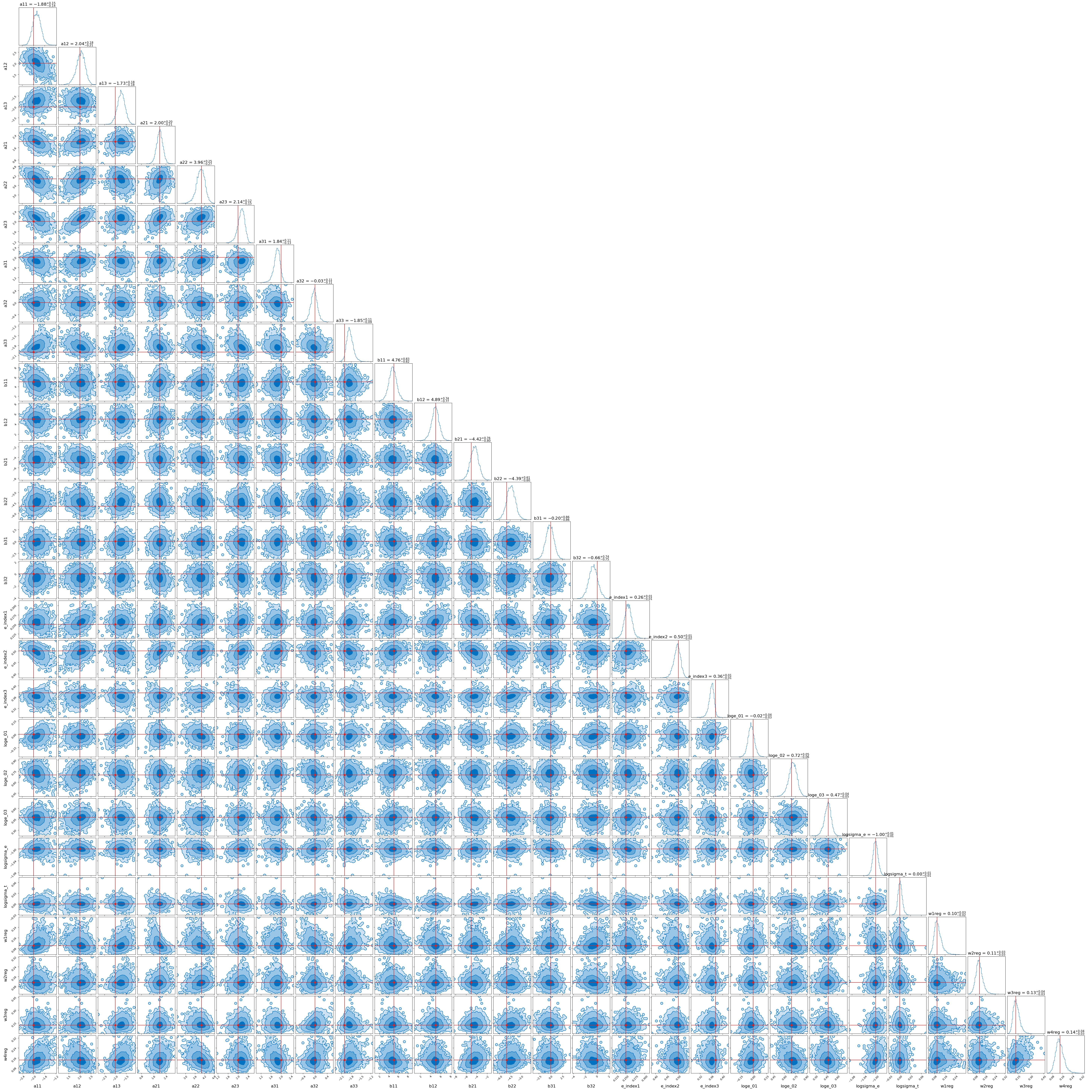
Here’s the final result (with slightly different data, hence the extra mixture). It only took 10 minutes but I let it run for a little longer than I needed to so that I was sure the result was stable.

And the code

import numpyro
import numpyro.distributions as dist
from numpyro.handlers import scale
import jax.numpy as jnp
from numpyro.infer.autoguide import AutoDiagonalNormal, AutoMultivariateNormal, AutoBNAFNormal, AutoIAFNormal
from numpyro.infer.initialization import init_to_uniform
from numpyro.infer import SVI, Trace_ELBO
from numpyro.optim import Adam
from tqdm import tqdm
import jax


def model_svi_flow():
    a11 = numpyro.sample("a11", dist.Normal(aloc+ascale/2, ascale/5))
    a12 = numpyro.sample("a12", dist.Normal(aloc+ascale/2, ascale/5))
    a13 = numpyro.sample("a13", dist.Normal(aloc+ascale/2, ascale/5))

    a21 = numpyro.sample("a21", dist.Normal(aloc+ascale/2, ascale/5))
    a22 = numpyro.sample("a22", dist.Normal(aloc+ascale/2, ascale/5))
    a23 = numpyro.sample("a23", dist.Normal(aloc+ascale/2, ascale/5))

    a31 = numpyro.sample("a31", dist.Normal(aloc+ascale/2, ascale/5))
    a32 = numpyro.sample("a32", dist.Normal(aloc+ascale/2, ascale/5))
    a33 = numpyro.sample("a33", dist.Normal(aloc+ascale/2, ascale/5))

    b11 = numpyro.sample("b11", dist.Normal(bloc+bscale/2, bscale/5))
    b12 = numpyro.sample("b12", dist.Normal(bloc+bscale/2, bscale/5))

    b21 = numpyro.sample("b21", dist.Normal(bloc+bscale/2, bscale/5))
    b22 = numpyro.sample("b22", dist.Normal(bloc+bscale/2, bscale/5))
    
    b31 = numpyro.sample("b31", dist.Normal(bloc+bscale/2, bscale/5))
    b32 = numpyro.sample("b32", dist.Normal(bloc+bscale/2, bscale/5))


    loge_01 = numpyro.sample("loge_01", dist.Normal(loge0_loc+loge0_scale/2, loge0_scale/5))
    loge_02 = numpyro.sample("loge_02", dist.Normal(loge0_loc+loge0_scale/2, loge0_scale/5))
    loge_03 = numpyro.sample("loge_03", dist.Normal(loge0_loc+loge0_scale/2, loge0_scale/5))

    e_index1 = numpyro.sample("e_index1", dist.Normal(e_index_loc+e_index_scale/2, e_index_scale/5))
    e_index2 = numpyro.sample("e_index2", dist.Normal(e_index_loc+e_index_scale/2, e_index_scale/5))
    e_index3 = numpyro.sample("e_index3", dist.Normal(e_index_loc+e_index_scale/2, e_index_scale/5))


    logsigma_e = numpyro.sample("logsigma_e", dist.Normal(logsigma_e_loc+logsigma_e_scale/2, logsigma_e_scale/5))
    logsigma_t = numpyro.sample("logsigma_t", dist.Normal(logt_loc+logt_scale/2, logt_scale/5))


    w1reg = numpyro.sample("w1reg", dist.Uniform(0,1))
    w2reg = numpyro.sample("w2reg", dist.Uniform(0,1))
    w3reg = numpyro.sample("w3reg", dist.Uniform(0,1))
    w4reg = numpyro.sample("w4reg", dist.Uniform(0,1))


    theta_flow = jnp.array([a11, a12, a13, b11, b12, loge_01, e_index1, \
                        a21, a22, a23, b21, b22, loge_02, e_index2, \
                        a31, a32, a33, b31, b32, loge_03, e_index3, \
                        logsigma_t, logsigma_e, w1reg, w2reg, w3reg, w4reg])  

    # Add your custom log-likelihood
    unnormalised_posterior_val = unnormalised_posterior(theta_flow)

    numpyro.factor("unnormalised_posterior_val", unnormalised_posterior_val)



guide_flow = AutoIAFNormal(model_svi_flow, 
                            num_flows=8, 
                            hidden_dims=[50, 50])


svi_flow_optimizer = Adam(1e-3, b1=0.99, b2=0.999)
svi_flow_svi = SVI(model_svi_flow, guide_flow, svi_flow_optimizer, loss=Trace_ELBO(num_particles=50))

# Initialize and run
rng_key_svi_flow= jax.random.PRNGKey(0)
svi_state_svi_flow = svi_flow_svi.init(rng_key_svi_flow)

n_steps = 1400
num_save_skip = 20
param_history_svi_flow = []
elbo_history_svi_flow = []

for step in tqdm(range(n_steps)):
    svi_state_svi_flow, loss_svi_flow = svi_flow_svi.update(svi_state_svi_flow)

    if step % num_save_skip == 0:
        params_svi_flow = svi_flow_svi.get_params(svi_state_svi_flow)
        param_history_svi_flow.append(params_svi_flow)
        elbo_history_svi_flow.append(loss_svi_flow)