Practical Intro to the Metropolis-Hastings Algorithm/Fitting a line II

In this post, I’m going to try to give an intuitive intro into the Metropolis-Hastings algorithm without getting bogged down in much of the math to show the utility of this method.

Metropolis-Hastings (or more truthfully, the subsequent MCMC field) is one of the most successful analytical methods that statisticians have ever used and is the benchmark for all future analysis methods that we will explore. I am basing this tutorial on various sources, such as:

• 📝 A Conceptual Introduction to Markov Chain Monte Carlo Methods - Joshua S. Speagle
• 🌐 Markov chain Monte Carlo sampling - Andy Casey
• 🌐 The Wikipedia page on this topic is also very good: Metropolis–Hastings algorithm
• ▶️ Understanding Metropolis-Hastings algorithm - Machine Learning TV
• ▶️ The algorithm that (eventually) revolutionized statistics - #SoMEpi - Very Normal
  • I particularly connected with this one, so if this post seems too similar… sorry 😬
  • Although I was able to get my own algorithm to work 😬 (I have no idea why he went straight to 12 parameters…)
• ▶️ Metropolis-Hastings - VISUALLY EXPLAINED! - Kapil Sachdeva
• 🌐 The Metropolis-Hastings algorithm - Danielle Navarro
• 🌐 Why Metropolis–Hastings Works - Gregory Gundersen

If you don’t like or connect well with how I explain the concepts below, absolutely head over to any of these resources. They do widely vary in rigor and presentation method but are all great.

And the style of my GIFs is inspired by this video PDF Sampling: MCMC - Metropolis-Hastings algorithm - Ridlo W. Wibowo

Table of Contents

• Motivation
  • Brute force? In this economy?
• What do we actually get from our analysis?
  • Samples!?
  • How do we sample our posterior?
• Metropolis-Hastings algorithm - Dessert before dinner
  • The algorithm
• Coding it up…again
• Well… now what?

Motivation

Brute force? In this economy?

In the last post, we brute-forced our analysis by scanning the whole entire parameter space for areas of high posterior probability. Here’s a quick recap.

1. We were given some data that I told you was from a straight line with some added Gaussian noise.

   

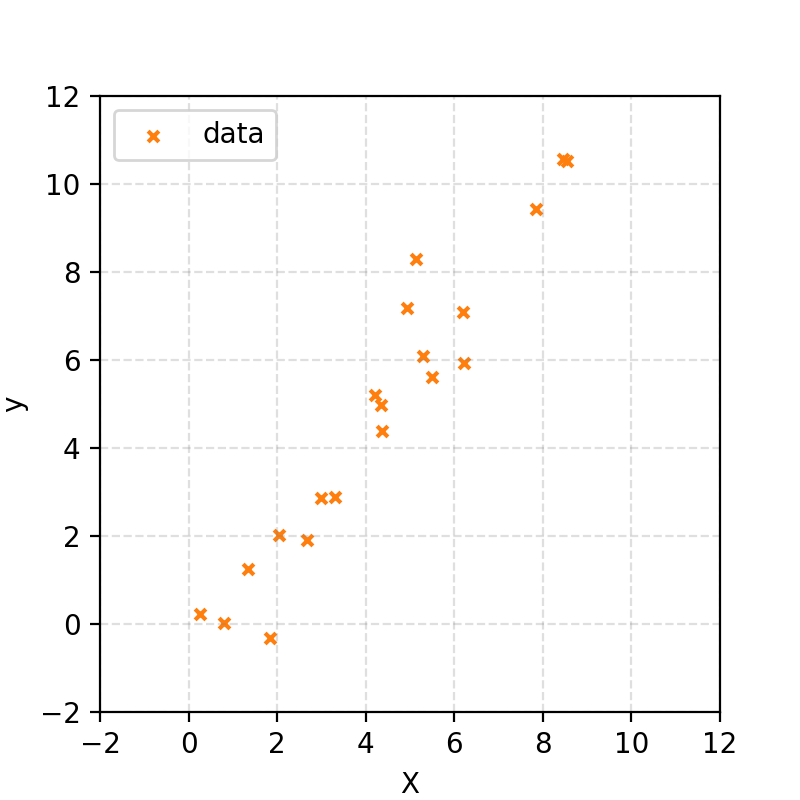
2. We then quantified a likelihood and a prior based on this information and produced something like this colormap of the posterior probabilities of the input parameters.

   

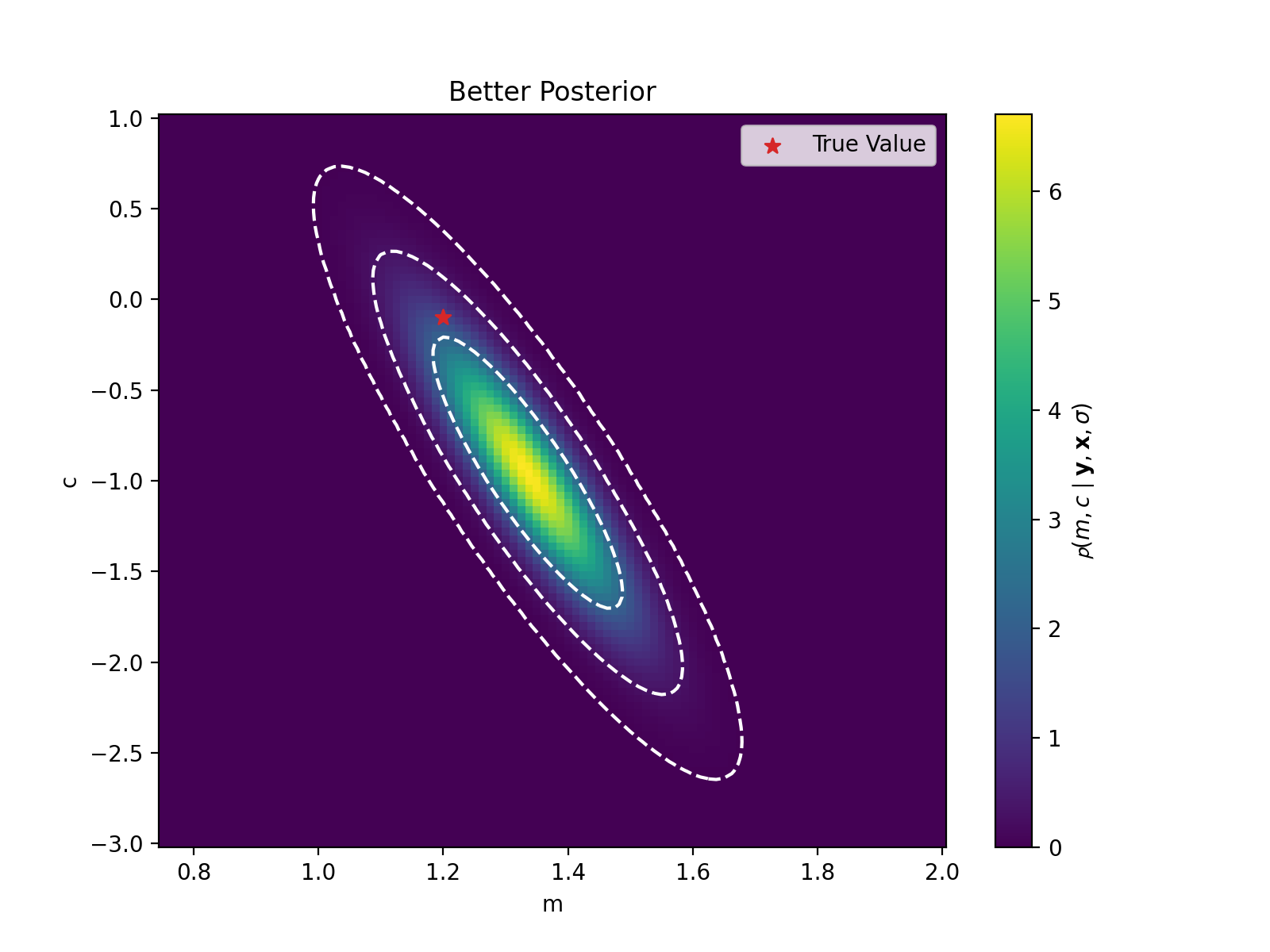
In most scenarios, this is infeasible (or at least expensive), and we need something more sophisticated to explore regions of high probability and somehow get some representation of our posterior. So, what could we do instead?

What do we actually get from our analysis?

If our goal is to get something representative of the posterior, we generally want to do one or more of the following:

1. Guess where the most optimal set of parameter values are based on our data (not unique to posterior inference; can just be done with optimization).
2. Generate further values that reflect parameter uncertainties.
3. Quantify uncertainty.
4. Compare models via evidence values (normalization for the posterior).

So whatever other method we use to generate something representative of the posterior, we need to keep these in mind¹.

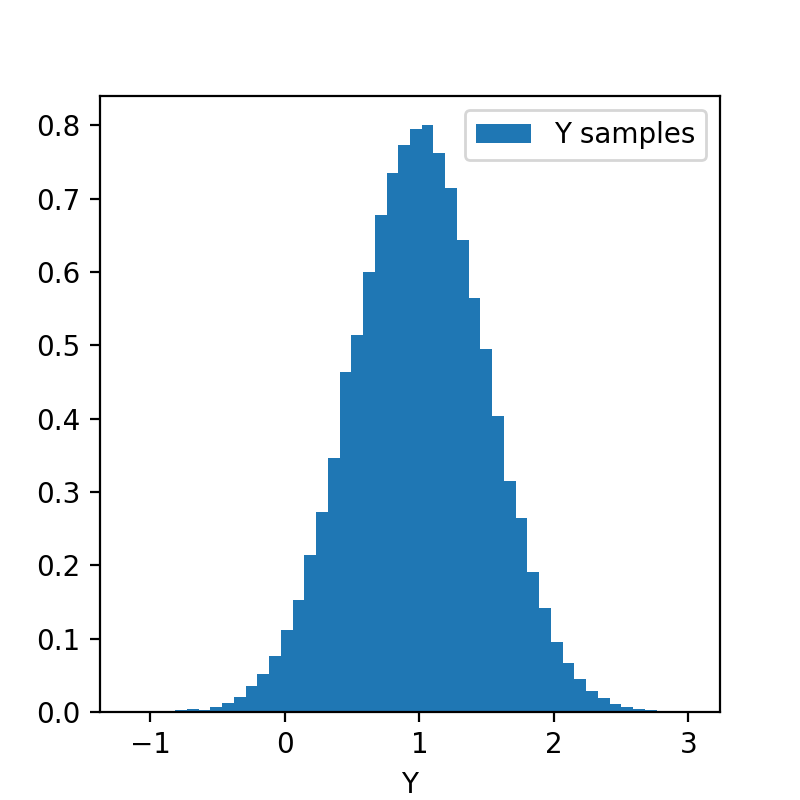
You are already familiar with another way that we often represent the results of analysis, that is through samples. For example, sure, I could tell you that for model X, parameter Y follows a normal distribution with a mean of 1 and a standard deviation of 0.5. (First of all, this only works if our result has a functional representation and we presume our audience even knows what a normal distribution is.) Or, we could show them a histogram of our results like the following.

from scipy.stats import norm
from matplotlib import pyplot as plt
import numpy as np


samples = norm(scale=0.5, loc=1).rvs(100000)


fig, ax = plt.subplots(1,1, figsize=(4,4), dpi=200)
ax.hist(samples, bins=48, label="Y samples", density=True)
ax.set_xlabel("Y")
ax.legend()
plt.show()

Samples!?

Now, if you tell anyone off the street that the parameter follows this distribution, they would be able to glean most of the key information (although I wouldn’t recommend pulling people off the street and asking them random statistics questions, by the way… you often don’t get the best responses. Unless the question is how many times can someone threaten your life in ~10 seconds, in which case it’s extremely informative…).

1. You can see where the mode of the distribution is.
2. We could generate further samples of variables by using the samples in this distribution and see the result.
3. You can see the spread of the distribution on the parameter to understand our uncertainty on it. (We can also construct credible intervals through various methods to get quantitative values for our uncertainties.)

And from these samples, we’ve also shown essentially the same information as our first brute scan colormap. What we require is a set of samples representative of the same probability density! This both reduces the initial computation cost, as we don’t have to explore regions of the parameter space where the probabilities are extremely small, and in the storage of the result, as we will likely only require \(\lesssim 100,000\) samples/numbers to show this.

We also don’t explicitly have a way to get evidence values for model comparison from this, but we can tackle this later if/when we look at Nested Sampling.

How do we sample our posterior?

Now, unlike the above normal distribution, our function isn’t normalized; we have the top part of the fraction that makes up Bayes’ theorem.

But from our perspective, \(\vec{d}\) is a constant, so we can say:

Now you might want to calculate \(\mathcal{Z}(\vec{d})\) directly but you would run into the same issues (and worse) when we tried to directly, but you would run into the same issues (and worse) when we tried to directly scan the posterior to begin with (this is further explored in Section 4 of Speagle’s introduction). So we need some method where we can sample something proportional to a probability density.

Metropolis-Hastings! - Having dessert before dinner

One answer to this is the Metropolis-Hastings algorithm. And like the heading I’m going to show you the end result so you can see why what we’re doing is so cool.

Using the unnormalized posterior function we used in the last post on line fitting, I’m going to create a pretty small function that will almost magically generate samples from our distribution.

import numpy as np
import matplotlib.pyplot as plt

# Metropolis-Hastings algorithm for 2D
def metropolis_hastings_function(posterior, data, num_samples, proposal_cov, start_point):
    samples = []
    current = np.array(start_point)
    for _ in range(num_samples):
        # Propose a new point using a 2D Gaussian
        proposal = np.random.multivariate_normal(current, proposal_cov)

        # Calculate acceptance probability
        acceptance_ratio = np.exp(posterior(*data, *proposal) -  posterior(*data, *current))

        # Cap at 1, gotta be a probability and probabilities can't be more than 1
            # Probability _densities_ can but those aren't _probabilities_ until you integrate them
        acceptance_ratio = min(1, acceptance_ratio)  

        # Accept or reject
        if np.random.rand() < acceptance_ratio:
            current = proposal

        samples.append(current)

    return np.array(samples)

# Parameters
num_samples = 50000
proposal_cov = [[0.1, 0], [0, 0.1]]  # Proposal covariance matrix
start_point = [m_true, c_true]  # Starting point for the chain

# Run Metropolis-Hastings
samples = metropolis_hastings_function(unnormalised_log_posterior_better, (y, X_true), num_samples, proposal_cov, start_point)

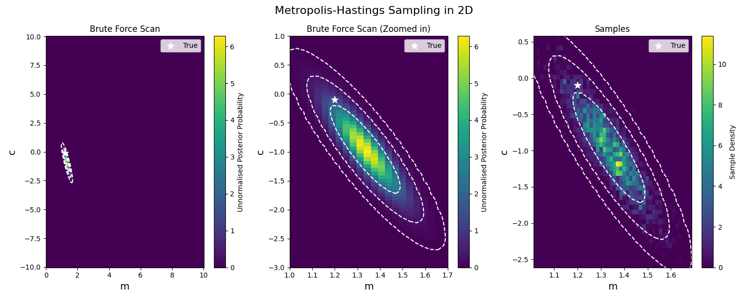
Magic! Now, it isn’t the prettiest thing, and to be fair to it, this algorithm is (recently, as of 2020) over 50 years old! And since then, there have been a lot of improvements, but isn’t it amazing that with so little code, we are able to do something like this? Additionally, with the samples, there’s a handy package called corner that allows us to have a closer look at our samples.

from corner import corner
default_kwargs = {'smooth': 0.9,
    'label_kwargs': {'fontsize': 16},
    'title_kwargs': {'fontsize': 16},
    'color': 'tab:blue',
    'truth_color': 'k',
    'levels': (0.3934693402873666,
    0.8646647167633873,
    0.9888910034617577,
    0.9996645373720975,
    0.999996273346828),
    'plot_density': True,
    'plot_datapoints': False,
    'fill_contours': True,
    'max_n_ticks': 4,
    'hist_kwargs':{'density':True},
    "smooth":0.9,
}

fig = plt.figure(figsize=(6, 6), dpi=200)
corner(samples, 
    fig=fig,
    bins=36,
    truths=[m_true, c_true,],
    titles=[r"$m$", r"$c$"],
    show_titles=True,
    **default_kwargs)
plt.show()

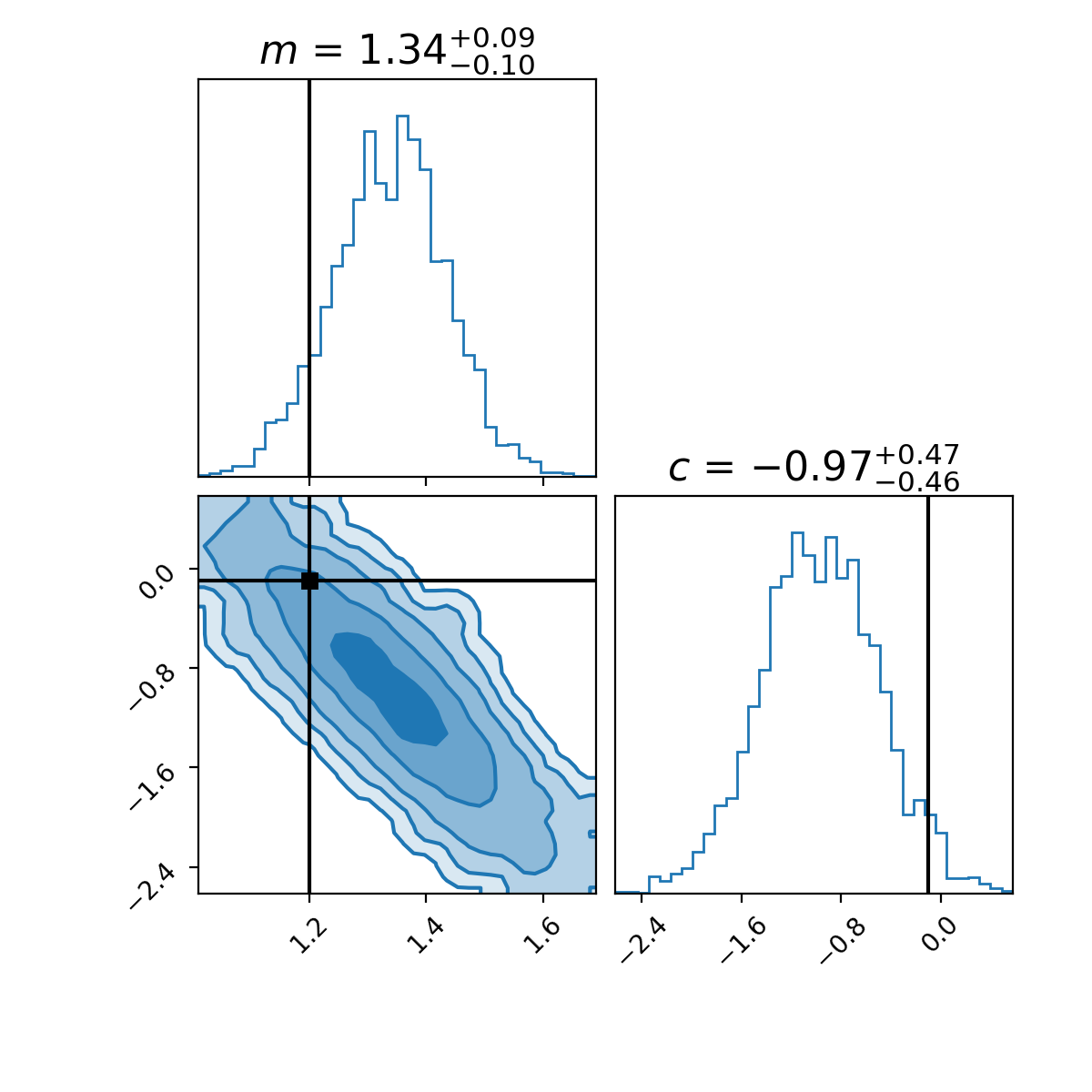
The top left and bottom right plots in the above show the marginal distributions of the relevant parameters. These plots effectively show distributions once you take the explicit dependence of the other variable(s) out¹. This is extremely useful when summarizing our results by text or by word we can’t show the plot, so we typically summarize our findings to one variable at a time, and further simplify it by asking what the width of the highest density region that contains the same area as a normal distribution between \(1\sigma\), \(2\sigma\), \(3\sigma\) (68%, 95%, 99.7%) or etc.

The algorithm

So here are the steps in plain-ish english.

Metropolis Algorithm

1. Initialise:
   1. Have a distribution you want to sample from (duh) \(f(x)\),
   2. manually create a starting point for the algorithm \(x_0\),
   3. pick a symmetric distribution \(g(x\mid y)\) to sample from
      • like a gaussian with a fixed covariance matrix such that \(g(x\mid y)=g(y\mid x)\)
   4. pick the number of samples you can be bothered waiting for \(N\)
2. For each iteration \(n\)/Repeat \(N\) times
   1. Sample a new proposal point \(x^*\) from the symmetric distribution centred at the previous sample
   2. Calculate the acceptance probability \(\alpha\) given as \(\alpha = f(x^*)/f(x_n)\)
      • And if the acceptance probability is more than 1, cap it at 1.
   3. Generate a number, \(u\), from a uniform distribution between 0 and 1
   4. Accept or reject²
      1. Accept if: \(u\leq\alpha\), s.t. \(x_{n+1} = x^*\)
      2. Reject if: \(u>\alpha\), s.t. \(x_{n+1} = x_n\)

The first thing to notice is that we don’t require the normalization of our function, as it just depends on the ratios, and the normalization cancels itself out. The second is that it doesn’t have many steps, despite being able to do quite a lot.

Now, this is the point that I want to show you an animation of the process, but I don’t want to do that with the 2D distribution as it’s slow enough as it is, and it would be annoying figuring out how to nicely visualize accepting or rejecting a sample. So, forgive me for doing this for a single-dimensional Gaussian that I made up on the spot.

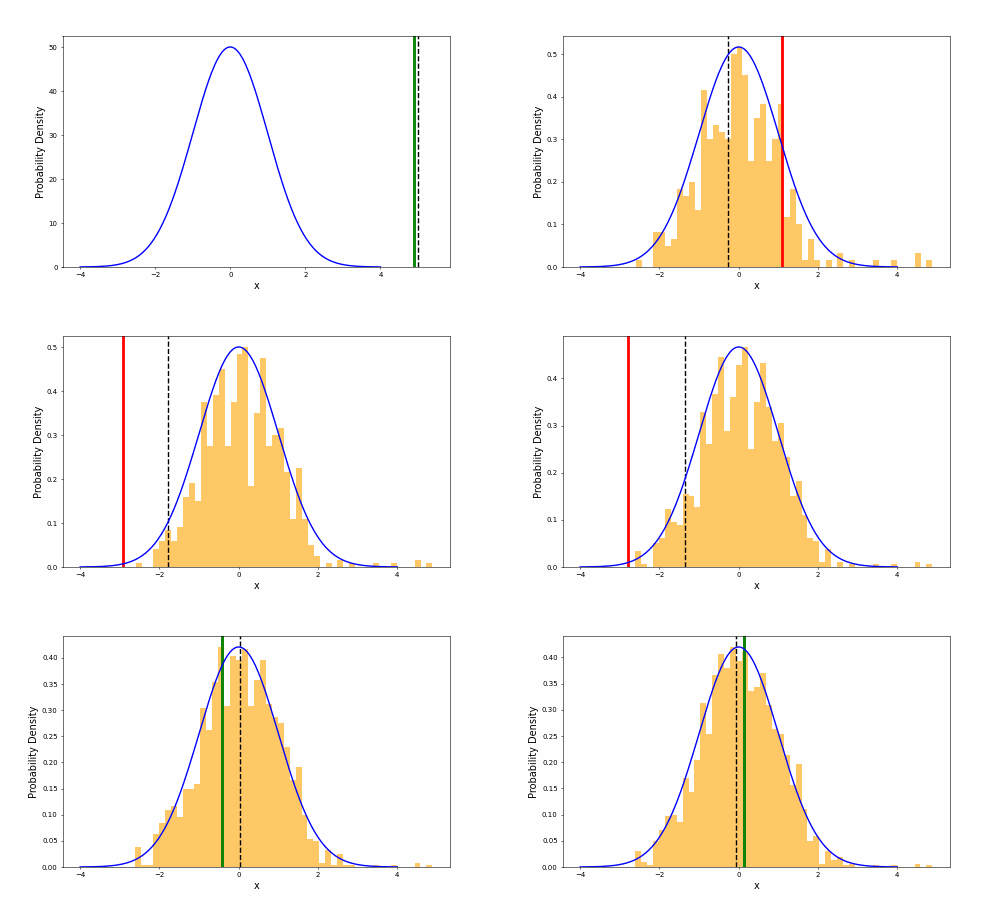
Slowing it down and having a look at the accepting conditions.

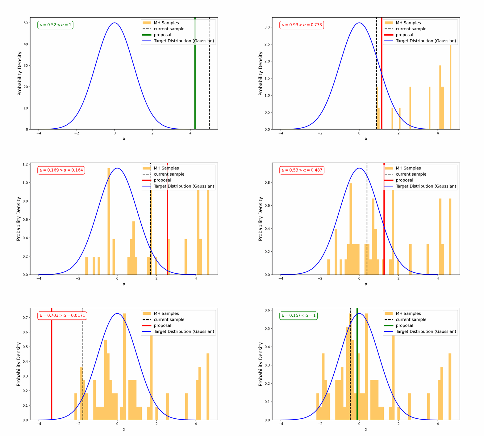
You will notice that in the GIF, there are some samples off to the side that don’t seem to fit the distribution. We refer to this as the “burn-in phase”; it is a sequence of samples at the beginning of MCMC sampling (not specific to Metropolis or the Metropolis-Hastings) where the chain of samples hasn’t reached the key part of the distribution yet. When doing your own MCMC sampling, you should be sure to throw away a few samples at the beginning³.

Very Normal had a great analogy for this process, because it may not be immediately intuitive why simply asking the ratio of two probabilities at a time allows us to construct the full probability distribution.

Let’s say you wanted to undertake the average distribution of activities that Melburnian’s undertake every week.

• You go to an activity around Melbourne that you think Melburnian’s undertake (initialisation)
• You do the activity
• After spending an amount of time at the activity you randomly pick an activity among a list of nearby ones that you are sure covers the whole range of activities that Melburnians undertake
• You then ask one of the natives whether they think they spend more time at the current activity or the random one you picked
• With a probability of the ratio of how much time they spend at each activity you either stay at your current activity or go to the new one
• Repeat

And eventually, even if you didn’t pick an activity that was very good, you will eventually be led to the “good” activities (equilibrium distribution) and start to do the same activities as typical Melburnians do, despite only ever comparing two choices at a time: “stay” or “next”.

However, if this decision process only allows transitions between certain activities (e.g., people who go to cafes only talk to others at cafes), then some activities might be overrepresented while others remain underexplored⁴.

This is an issue for the Metropolis algorithm⁵, which is what I detailed above, but not the generalisation of the algorithm by Wilfred Keith Hastings the Metropolis-Hastings algorithm.

For the Metropolis algorithm to work, we presume that the proposal distribution, \(g\), is symmetric, i.e. \(g(x\mid y)=g(y\mid x)\), but this can be restrictive. Some distributions that may produce faster convergence or better fit a particular posterior setup may not be symmetric. So Hastings generalized the result to allow this, by modifying the acceptance probability from \(\alpha = f(x^*)/f(x_n)\) to \(\alpha = \frac{f(x^*)g(x_n\mid x^*)}{f(x_n)g(x^*\mid x_n)}\) which accounts for any assymetry in \(g\) (I’ll go into more detail in a later post).

Metropolis-Hastings Algorithm

1. Initialise:
   1. Have a distribution you want to sample from (duh) \(f(x)\),
   2. manually create a starting point for the algorithm \(x_0\),
   3. pick a distribution \(g(x\mid y)\) to sample from (now doesn’t need to be symmetric)
   4. pick the number of samples you can be bothered waiting for \(N\)
2. For each iteration \(n\)/Repeat \(N\) times
   1. Sample a new proposal point \(x^*\) from the syymetric distribution centred at the previous sample
   2. Calculate the acceptance probability \(\alpha\) given as \(\alpha = \frac{f(x^*)g(x_n\mid x^*)}{f(x_n)g(x^*\mid x_n)}\) (Here’s the change!)
      • And if the acceptance probability is more than 1, cap it at 1.
   3. Generate a number, \(u\), from a uniform distribution between 0 and 1
   4. Accept or reject²
      1. Accept if: \(u\leq\alpha\), s.t. \(x_{n+1} = x^*\)
      2. Reject if: \(u>\alpha\), s.t. \(x_{n+1} = x_n\)

Now we’ll see when an asymmetric proposal distribution can do better than a symmetric one; we’ll look at the two algorithms side-by-side⁶.

For the distribution that we’re trying to model, we’ll use the Gamma distribution with \(\alpha=2\) and our two proposal distributions will be a normal distribution with a standard deviation of 0.5 for our symmetric distribution and a log-normal distribution with \(\sigma=0.5\) for our asymmetric distribution.

Additionally, arviz can estimate the number of effective samples.

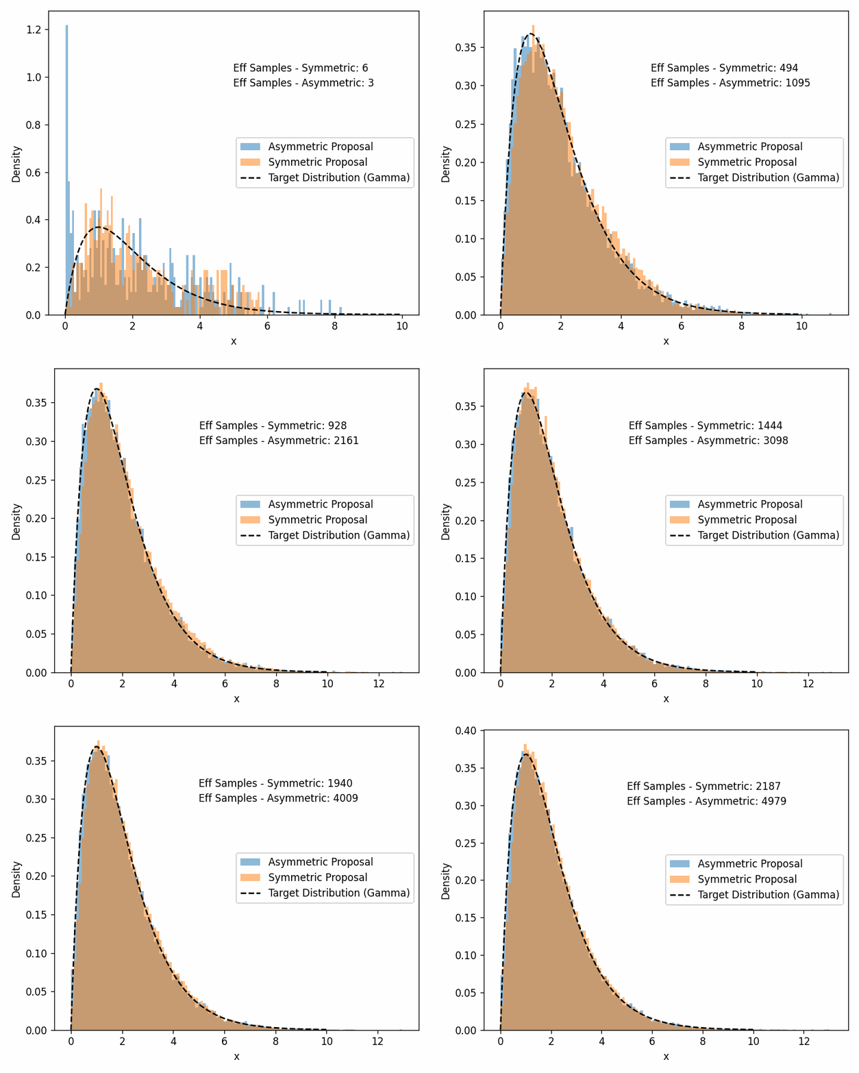
You can see that the asymmetric proposal distribution is able to get the core shape of the distribution more quickly than the symmetric distribution. Especially if you look at the left edge of the distribution and the tail past 7 or so.

Viva le estadistica⁷!… (looks up noun gender of statistics in Spanish)… Viva la estadistica⁸!

Coding it up … again

Just for completeness I’ll copy-paste my implementation of the Metropolis-Hastings algorithm here as well.

def metropolis_hastings(
        target_pdf, 
        proposal_sampler, 
        proposal_pdf, 
        num_samples=5000, 
        x_init=1.0):

    samples = [x_init]

    x = x_init

    for _ in range(num_samples):

        # Propose a new sample
        x_prime = proposal_sampler(x) 

        # Just for the gamma distribution to ensure positivity. 
            # I couldn't get it to work nicely without this
            # If _you_ wanna use this for something else, I would take this 
            # bad boi out or replace it with a relevant constraint for the 
            # distribution of interest
        if x_prime <= 0:  
            continue

        # Compute acceptance ratio \alpha = f(x^*)/f(x_n) * g(x_n|x^*)/g(x_^*|x_n)
        p_accept = (target_pdf(x_prime) / target_pdf(x)) \
        * proposal_pdf(x, scale=x_prime)/proposal_pdf(x_prime, scale=x)

        # Cap it, bop it, twist it
        p_accept = min(1, p_accept)

        # Simulate random process of accepting the proposed sample with probability p_accept
        if np.random.rand() < p_accept:
            x = x_prime
        # else: x = x

        samples.append(x)

    return np.array(samples)

A quick note

I’ve gone through the Metropolis-Hastings algorithm here and told you about burn-in, but there are other criteria for whether you should trust your samples/diagnostics. I’m going to leave that for another time as you will likely never use Metropolis-Hastings in practice but other algorithms, so I’ll talk about diagnostics there and after I introduce MCMC as a concept in general (which I haven’t so far).

Well… now what?

Next I’m going to attempt to explain what MCMC is in general and why detailed balance as a property of our MCMC algorithms is important and how we can quantify how we can judge whether our samples have converged and later to maybe give a general intro into the now much more commonly used NUTS algorithm that most MCMC python packages like emcee, pyMC and many others use.