Rejection Sampling

In this post I’m going to introduce rejection sampling as a way to generate samples from an unnormalised pdf as further background to MCMC.

Like my posts so far, I take heavy inspiration from a few resources. In this case, the in particular ones are:

1. Accept-Reject Sampling : Data Science Concepts - ritvikmath
2. An introduction to rejection sampling - Ben Lambert
   • Although this one is icky because he uses mathematica
3. Rejection Sampling - VISUALLY EXPLAINED with EXAMPLES! by Kapil Sachdeva

Table of Contents

• Intuition Introduction
  • Further Examples with uniform distribution
  • Using a more informative base distribution
• Math Intro
• Next Steps

Intuition Introduction

Let’s begin with the same kind of function as in my previous post on Inverse Transform Sampling (IVS).

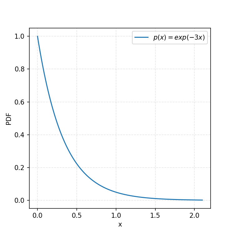
Similar to IVS, presuming that we can generate uniform samples between any two finite bounds, how can we produce an algorithm to give us samples of chosen PDF?

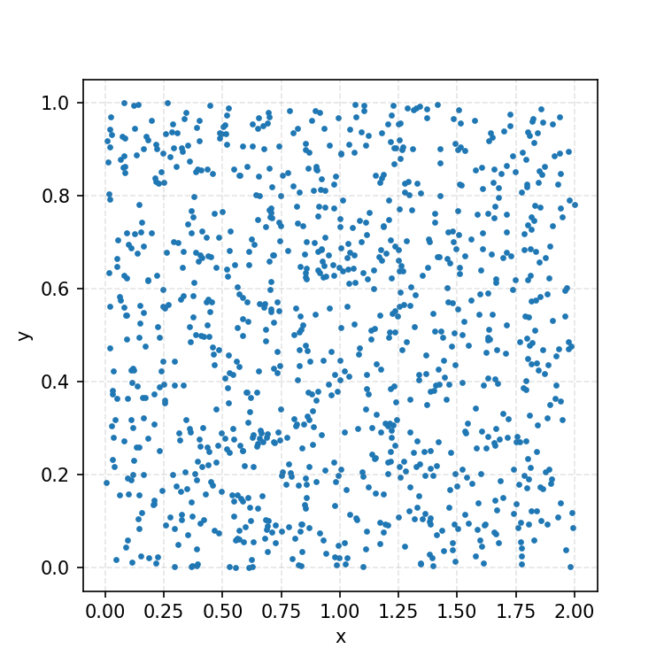
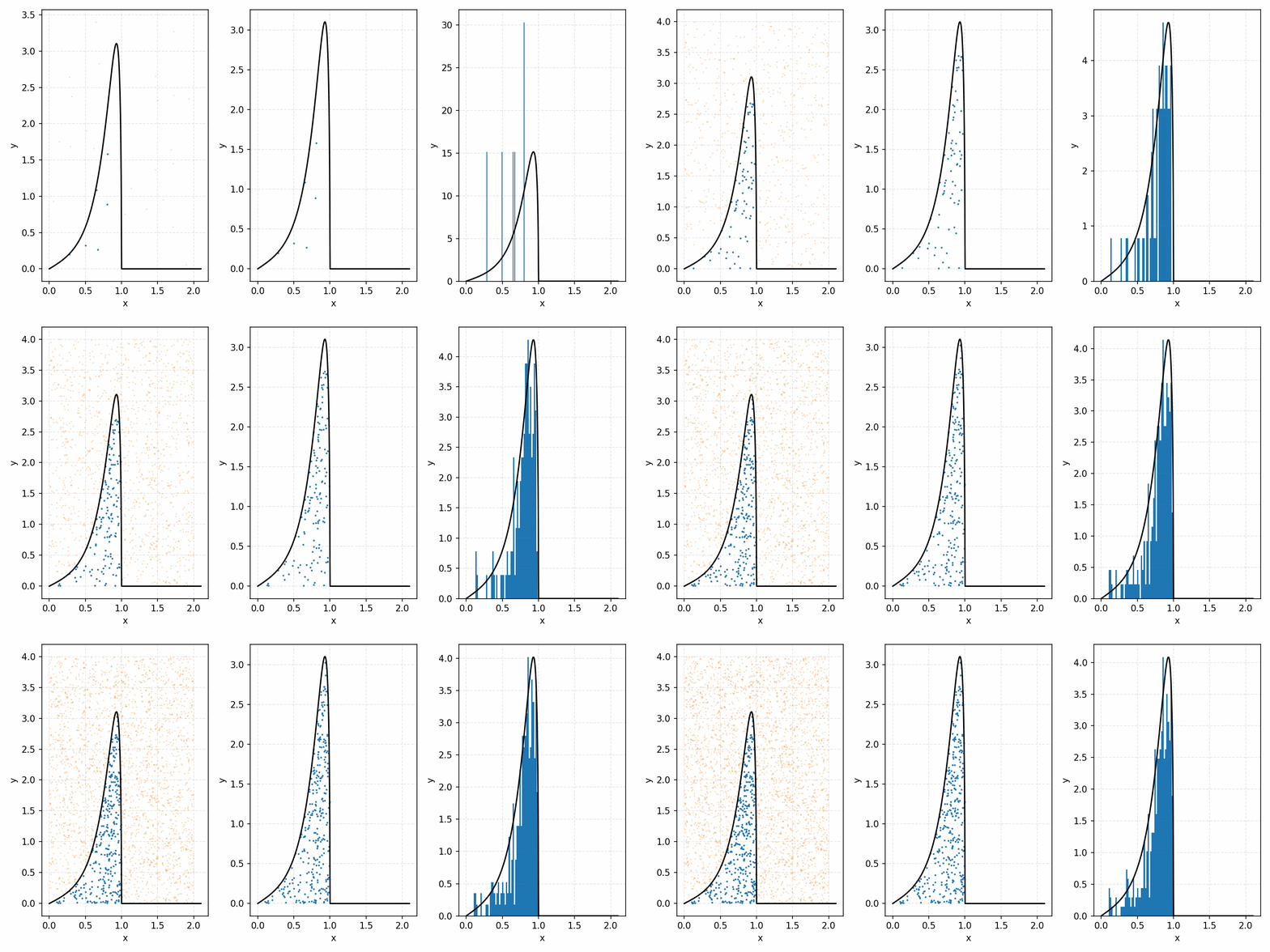
One thing you could do for the case above is produce samples between 0 and 2 for \(x\) and 0 to 1 for \(y\), producing the below scatter plot.

We then overlay our pdf and the samples.

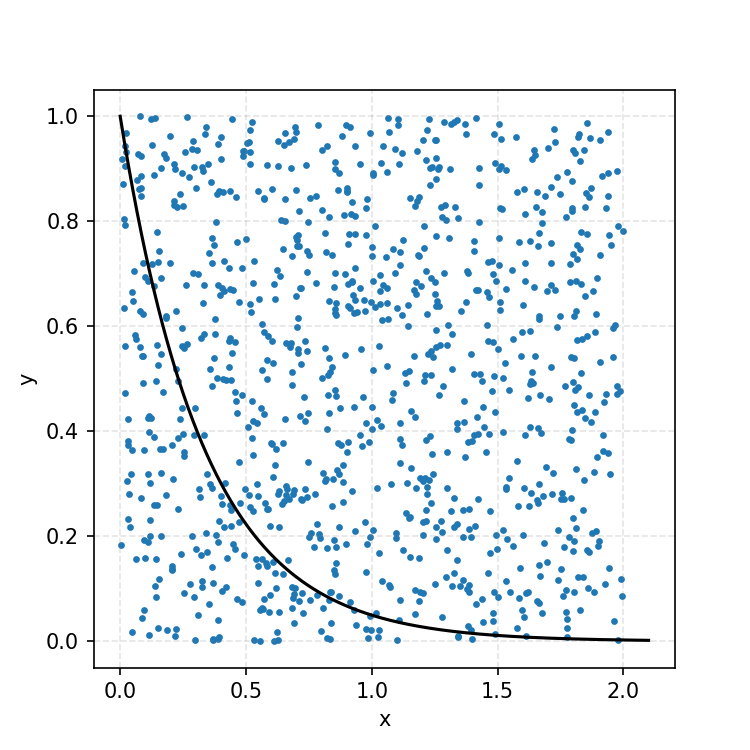
Then, you can think of what we have as a dot plot, and throw out samples above our pdf.

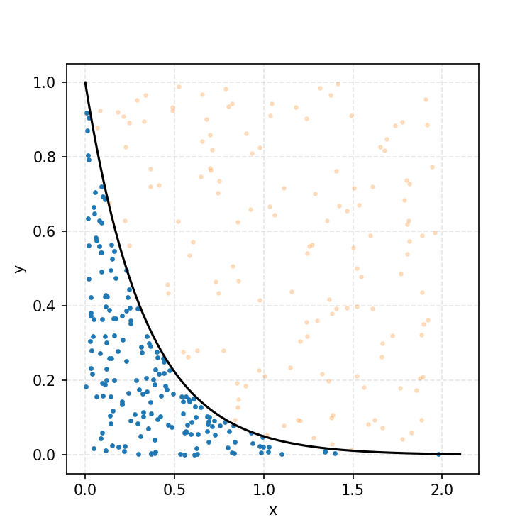
Converting these samples into a histogram we then find the following.

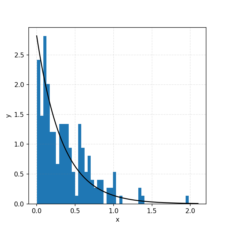
Which you can see is following the right curve but let’s increase the number of samples to be sure.

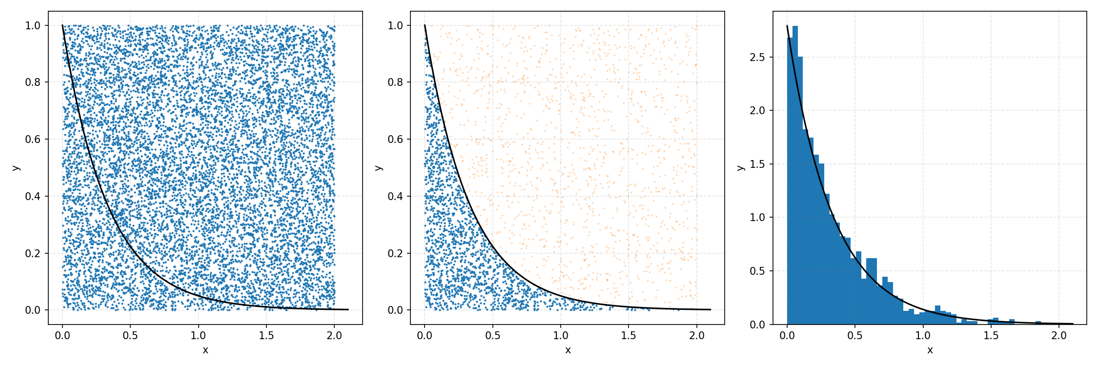
And that’s the basic idea of Rejection Sampling.

This base form is obviously extremely inefficient at producing exact representative samples as opposed to Inverse Transform Sampling. However, it is easier to implement for multi-dimensional distributions and when you can’t rigorously normalise the PDF (either due to dimensionality or stability). The only requirement is that you have some \(M\) such that \(PDF(x)<M*f(x)\) where \(g(x)\) is your proposal distribution (so far, a uniform distribution which is just a constant value) for all \(x\). In the previous case \(M=1\), but we could also have used 2 or anything higher if we wanted, it would just be less efficient as we would be wasting more samples.

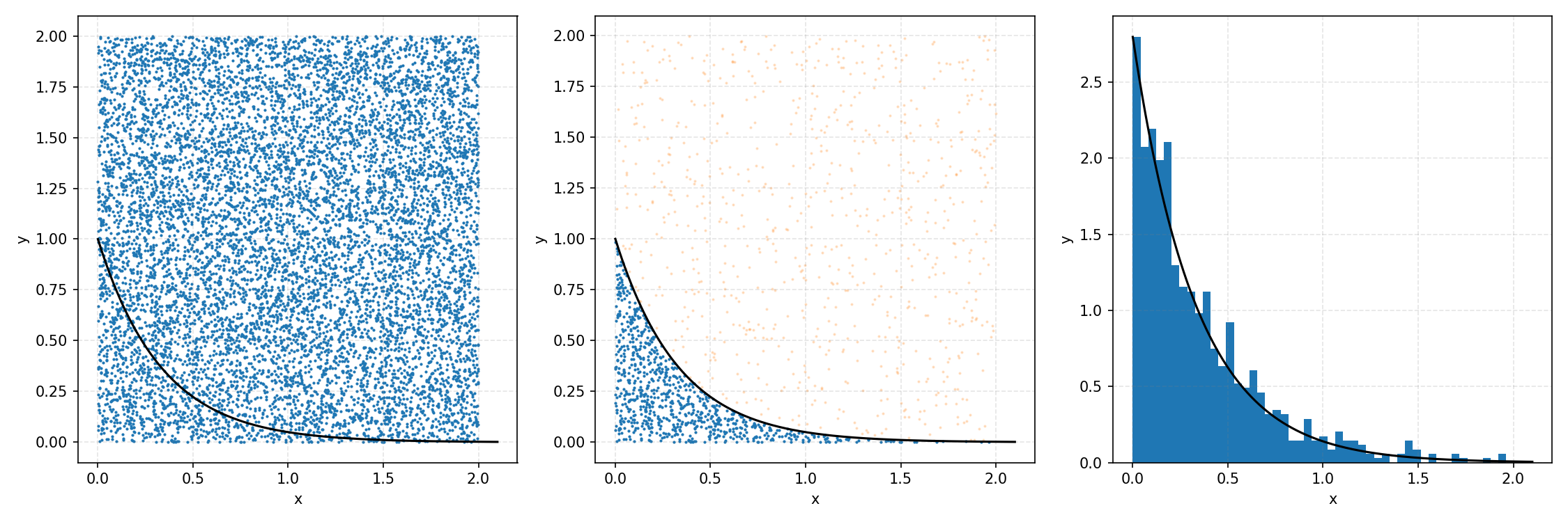
Here’s the code to produce the plots for \(M=1\).

import numpy as np
from matplotlib import pyplot as plt
from scipy.stats import uniform

lambda_val = 3

# Choose the number of samples
num_samples = int(1e4)

# Sample X uniformly between 0 and 2
uniform_x_samples = uniform(loc=0, scale=2).rvs(num_samples)

# Sample Y uniformly between 0 and 1
uniform_y_samples = uniform(0, 1).rvs(num_samples)



fig, ax = plt.subplots(1, 3, figsize=(15, 5), dpi=150)

ax = np.array(ax).flatten()

## Producing plot with overlay of uniform samples and PDF
ax[0].scatter(uniform_x_samples, uniform_y_samples, s=1)
ax[0].set_ylabel("y")
ax[0].set_xlabel("x")
ax[0].grid(ls='--', c='grey', alpha=0.2)


ax[0].plot(x_inputs, exp_func(x_inputs, lambda_val), label=r"$p(x) = exp(-$"+f"{lambda_val}"+r"$x)$", c='k')


## Producing plot with rejected samples
ax[1].plot(x_inputs, exp_func(x_inputs, lambda_val), label=r"$p(x) = exp(-$"+f"{lambda_val}"+r"$x)$", c='k')

# Find indices of samples where y_i < PDF(x_i)
good_point_indices = np.where(uniform_y_samples<exp_func(uniform_x_samples, lambda_val))[0]

# Look at samples that don't satisfy criterion and reduce their opacity
ax[1].scatter(uniform_x_samples[~good_point_indices], uniform_y_samples[~good_point_indices], s=1, label='bad samples', alpha=0.2, c='tab:orange')

# Look at samples that do satisfy criterion 
ax[1].scatter(uniform_x_samples[good_point_indices], uniform_y_samples[good_point_indices], s=1, label='good samples', c='tab:blue')


ax[1].set_ylabel("y")
ax[1].set_xlabel("x")
ax[1].grid(ls='--', c='grey', alpha=0.2)



## Producing the histogram
good_point_indices = np.where(uniform_y_samples<exp_func(uniform_x_samples, lambda_val))[0]

hist_output = ax[2].hist(uniform_x_samples[good_point_indices], label='good samples', density=True, bins=48)

func_vals = exp_func(x_inputs, lambda_val)
ax[2].plot(x_inputs, np.max(hist_output[0][:-5])*func_vals/np.max(func_vals[:-5]), label=r"$p(x) = exp(-$"+f"{lambda_val}"+r"$x)$", c='k')

ax[2].set_ylabel("y")
ax[2].set_xlabel("x")
ax[2].grid(ls='--', c='grey', alpha=0.2)
plt.tight_layout()
plt.show()

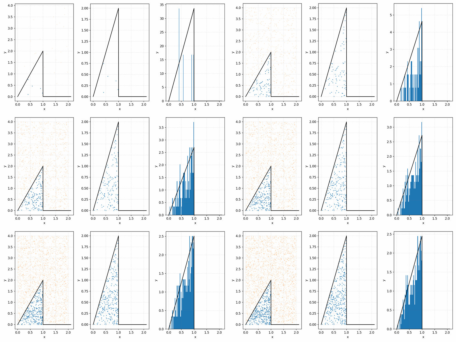
Further Examples with uniform distribution

Using a more informative base distribution

A little extension to this concept is that we do not need to simply sample a uniform distribution for \(Y\), we can sample any distribution \(g(x)\) such that \(g(x)\) is larger than our target \(p(x)\) for all x¹.

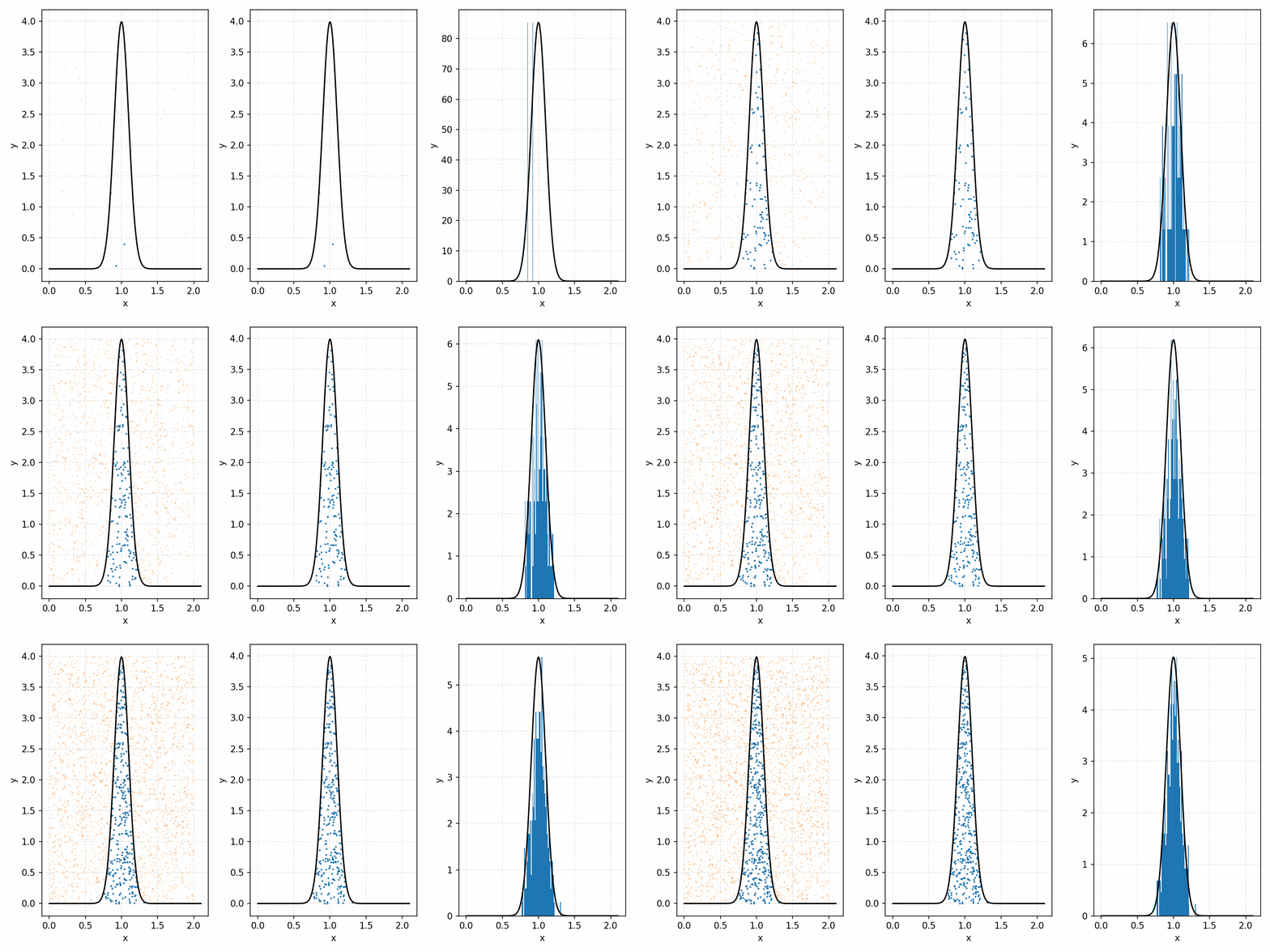
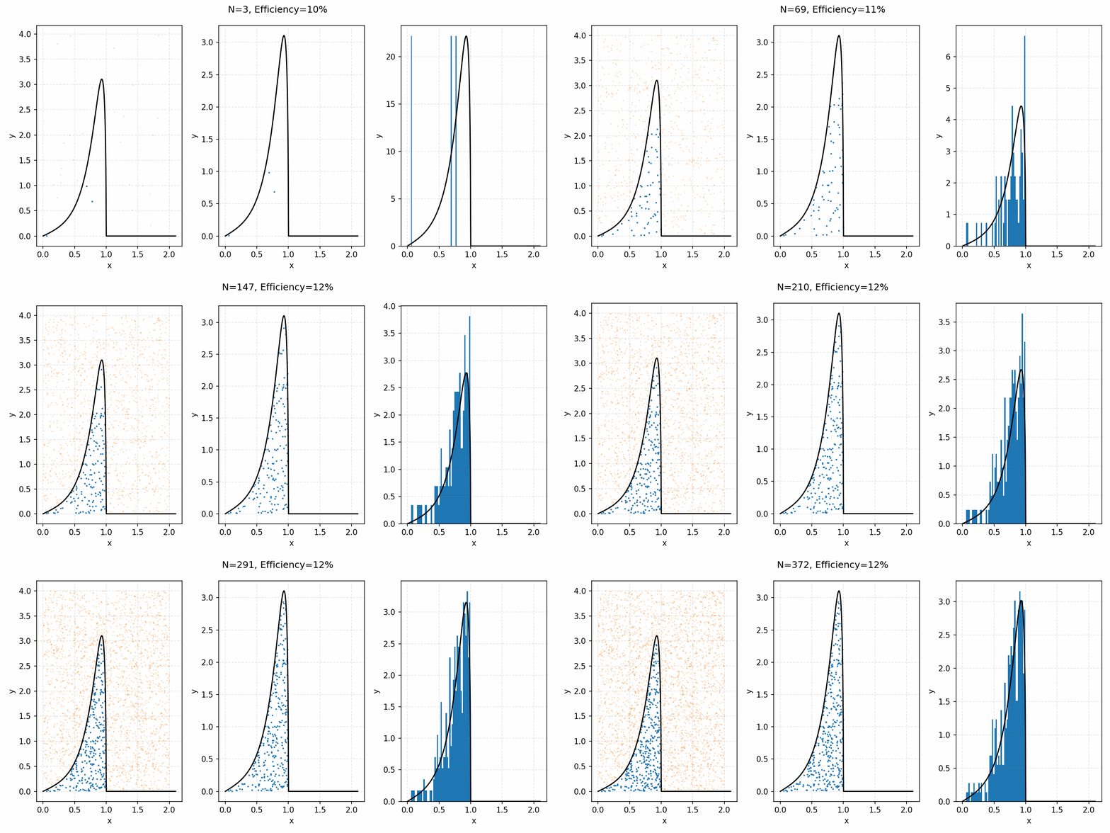
For example with the ARGUS distribution sampling shown below, you can see that there is a huge number of wasted samples. But you could imagine repeating the process by enveloping the distribution with a gaussian, sampling that, and then doing the same accept-reject algorithm as we did with the uniform distribution.

i.e. The algorithm is

1. Generate samples from a gaussian that is >= ARGUS for input values
2. Sample the same number of uniformly distributed values between 0 and 1.
3. If the proposal distributions probability times the uniform sample is \(\leq\) to the ARGUS pdf value for that input, accept it. If not, reject it.
   • This equivalent to accepting a sample with the probability \(PDF(x)/Proposal(x)\). More on this in the math-y introduction

Here’s a GIF showing the process.

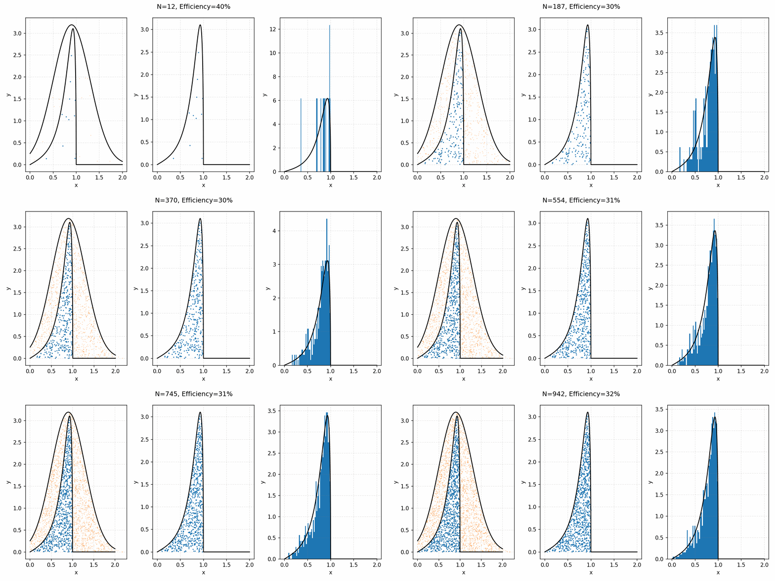
And we’ve tripled the efficiency!² You can further see this as the number of effective samples of the target distribution (\(N\)) is roughly three times the number than when we were sampling with the uniform distribution (and I’ve used the same number of total samples).

Here’s the code to make the same GIF.

import numpy as np
from matplotlib import pyplot as plt
from scipy.stats import uniform, norm, argus
import os

x_inputs = np.linspace(0.0001, 1.9999, 1001)
pdf_func = argus(chi=2.5).pdf
proposal_func = lambda x: 3.2*norm(loc=0.9, scale=0.4).pdf(x)

num_samples = int(3e3)
num_batches = 100
batch_size = num_samples//num_batches

proposal_x_samples = norm(loc=0.9, scale=0.4).rvs(num_samples)
proposal_y_samples = proposal_func(proposal_x_samples)*uniform(0, 1).rvs(num_samples)

png_dir = "argus_GIF_Pics_Better_Proposal"
os.makedirs(png_dir, exist_ok=True)
os.system(f"rm -rf {png_dir}/*.png")


for batch_idx in range(num_batches):

    batch_y_samples = proposal_y_samples[:(batch_idx+1)*batch_size][np.where(proposal_x_samples[:(batch_idx+1)*batch_size]>0)[0]]
    batch_x_samples = proposal_x_samples[:(batch_idx+1)*batch_size][np.where(proposal_x_samples[:(batch_idx+1)*batch_size]>0)[0]]

    fig, ax = plt.subplots(1, 3, figsize=(10, 5), dpi=150)

    ax = np.array(ax).flatten()

    ## Producing plot with overlay of uniform samples and PDF

    good_point_indices = np.where(batch_y_samples<pdf_func(batch_x_samples))[0]


    ax[0].scatter(batch_x_samples, batch_y_samples, s=1, label='bad samples', alpha=0.2, c='tab:orange')
    ax[0].scatter(batch_x_samples[good_point_indices], batch_y_samples[good_point_indices], s=1, label='good samples', c='tab:blue')

    ax[0].set_ylabel("y")
    ax[0].set_xlabel("x")
    ax[0].grid(ls='--', c='grey', alpha=0.2)


    ax[0].plot(x_inputs, pdf_func(x_inputs), c='k')
    ax[0].plot(x_inputs, proposal_func(x_inputs), c='k')


    ## Producing plot with rejected samples
    ax[1].plot(x_inputs, pdf_func(x_inputs), c='k')


    good_point_indices = np.where(batch_y_samples<pdf_func(batch_x_samples))[0]

    # ax[1].scatter(proposal_x_samples[~good_point_indices], proposal_y_samples[~good_point_indices], s=1, label='bad samples', alpha=0.2, c='tab:orange')
    ax[1].scatter(batch_x_samples[good_point_indices], batch_y_samples[good_point_indices], s=1, label='good samples', c='tab:blue')


    ax[1].set_ylabel("y")
    ax[1].set_xlabel("x")
    ax[1].grid(ls='--', c='grey', alpha=0.2)



    ## Producing the histogram
    good_point_indices = np.where(batch_y_samples<pdf_func(batch_x_samples))[0]

    hist_output = ax[2].hist(batch_x_samples[good_point_indices], label='good samples', density=True, bins=48)

    func_vals = pdf_func(x_inputs)
    ax[2].plot(x_inputs, np.max(hist_output[0][:-5])*func_vals/np.max(func_vals[:-5]), c='k')

    ax[2].set_ylabel("y")
    ax[2].set_xlabel("x")
    ax[2].grid(ls='--', c='grey', alpha=0.2)
    plt.suptitle(f"N={len(batch_y_samples[good_point_indices])}, Efficiency={100*len(batch_y_samples[good_point_indices])/len(batch_y_samples):.2g}%")
    
    plt.tight_layout()

    plt.savefig(f"{png_dir}/{batch_idx}.png")
    plt.close()


from PIL import Image
import os

# Output GIF file
output_gif = "argus_dist_with_better_proposal.gif"

# Get a sorted list of PNG files
png_files = sorted([f for f in os.listdir(png_dir) if f.endswith(".png")], key=lambda x: int(x.split('.')[0]))

# Create a list of images
images = [Image.open(os.path.join(png_dir, f)) for f in png_files]

# Save as a GIF
images[0].save(
    output_gif,
    save_all=True,
    append_images=images[1:],
    duration=120,  # Duration of each frame in milliseconds
    loop=0  # Loop forever; set to `1` for playing once
)

More mathematical introduction

Thanks again to ritvikmath for his work. This particular section is heavily influenced by his own video on the topic.

Our goal here is to be sure that the probability density of our samples, \(D(x\mid A)\)³, matches that of our target distribution, \(p(x)\), which we have in the unnormalised form of \(f(x)\).

As I hinted at when talking about generating samples from a more appropriate density/envelope, we can summarise our algorithm in another way.

1. Sample a value \(x\) from our proposal distribution \(g(x)\)
2. Accept this value with a probability of \(\mathcal{L}(A\mid x) = \frac{f(x)}{M\cdot g(x)}\)

Where when we were generating samples we instead multiplied a set of uniform values by \(M\cdot g(x)\) as a substitute for the second step.

With our new algorithm, using Bayes’ theorem (which I discussed in my line fitting blog post) we find that

Remembering that \(M\) is the value that we multiply our proposal density by such that \(M\cdot g(x) \geq p(x)\) for all x. So now the question is \(\mathcal{Z}(A)\)?

We can imagine that the purpose of \(\mathcal{Z}(A)\) is a normalisation constant so that the numerator becomes a probability density. i.e. So that we can integrate the right hand side over the range of parameter values and get 1. \(\mathcal{Z}(A)\) is a constant with respect to \(x\), so it needs to be whatever the integral of \(\frac{1}{M} f(x)\) is over x⁴.

Where I’ve introduced \(C\) as the normalisation constant on \(f(x)\) such that \(f(x)/C = p(x)\).

Therefore,

Woo! And if this all still doesn’t satisfy you here’s a link to where ritvikmath adds a bit more of a personal intuition.

Next Steps

So, one of the beautiful things we’ve done here is created a method where we can get an exact representation for any given sample distribution, but there are quite a few hiccups for why this isn’t used very much in practice as opposed to something like MCMC when trying to draw samples from a posterior distribution.

The main reason that we don’t often use these methods is we never know (or don’t presume to know) the exact shape of our posterior distribution⁵. So we can’t pick a very good proposal distribution, or pick one at all, meaning that we have to use something like a uniform distribution that we would have to update every call where we find a probability density higher than it’s max value, and update all our previous samples.

1. This is very inefficient especially with distributions that have a high dimensionality as we’ll inevitably be sampling regions with extremely low probabilities
2. This could be extremely expensive because we not only have to keep the samples that we are accepting, but also the ones that we aren’t, because we may update the distribution such that the acceptance/rejection of a sample changes

So, in the next post I’ll go through one of the most commonly used algoriths ever, and one of the most widely successful statistical algorithm ever, to explore unknown posterior densities when we have the likelihood and prior, the MCMC Metropolis-Hastings algorithm.