Inverse Transform Sampling
Published:
Introduction to inverse transform sampling for continuous and discrete probability distributions.
Introduction
The end goal of the next few posts is to build up to an intuitive understanding of how Markov Chain Monte Carlo (MCMC) methods work, following a similar method as the YouTuber ritvikmath’s videos on the topic.
At the heart of MCMC is a sampling algorithm for probability distributions with an unknown normalizing constant. In this tutorial, we will see how one can sample a probability density/mass distribution when you have the explicit form of the distribution.
Table of Contents
The End Result
If you’re short on time, this will be the only section that you need to look at. A general understanding of this topic will allow us to move on to future topics in Rejection Sampling and MCMC methods.
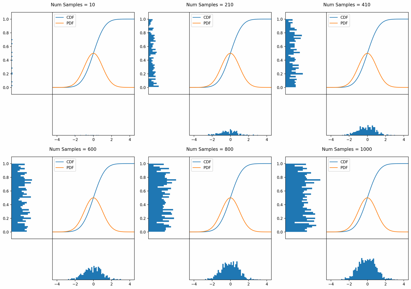
Let’s say you have a normal probability distribution function (pdf) and its cumulative distribution function (cdf). From the GIF below, you can see that if we invert the cdf and plug in some uniform samples from 0 to 1, then we get samples representative of the normal probability distribution.
And we can do this with any analytic continuous distribution. For example, below I have examples with a power law distribution, gamma distribution, ARGUS distribution, and others using scipy functions (the explicit functions aren’t important, just that you can see that the samples gradually mimic the pdf of the relevant distribution).
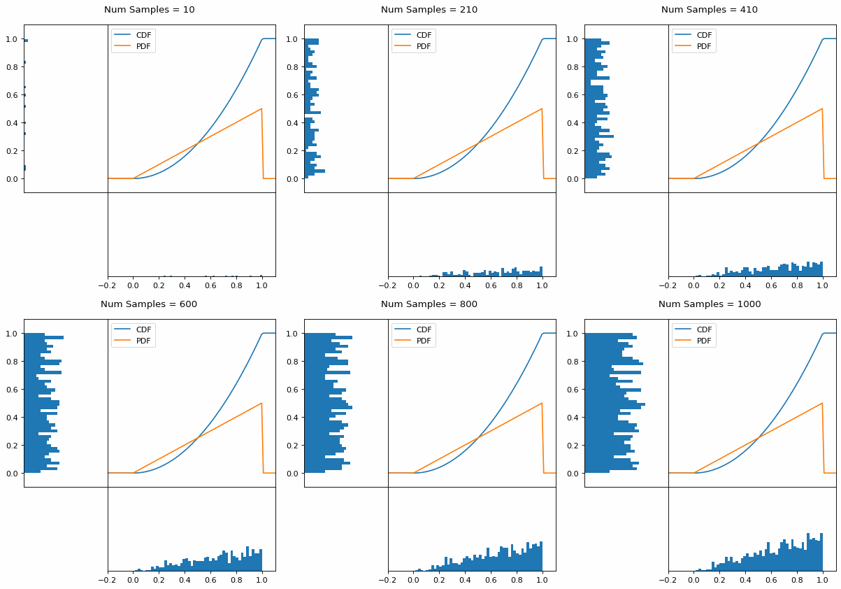
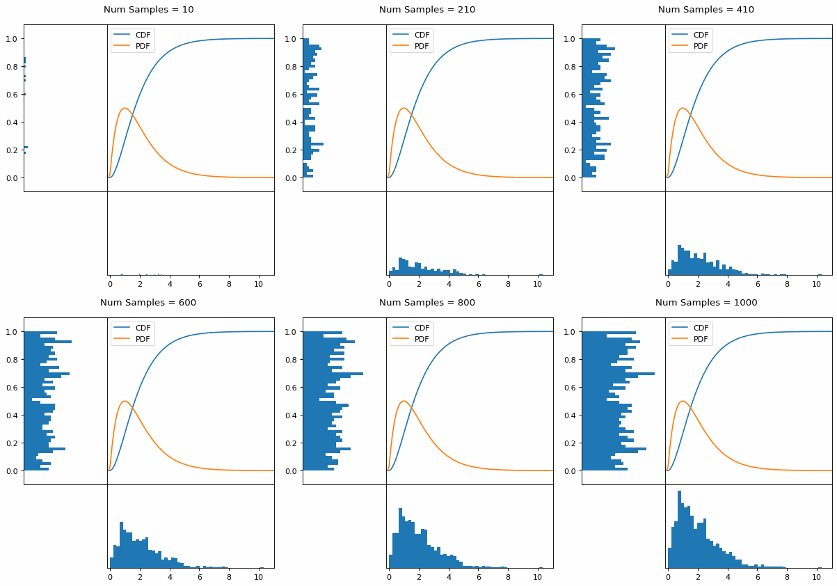
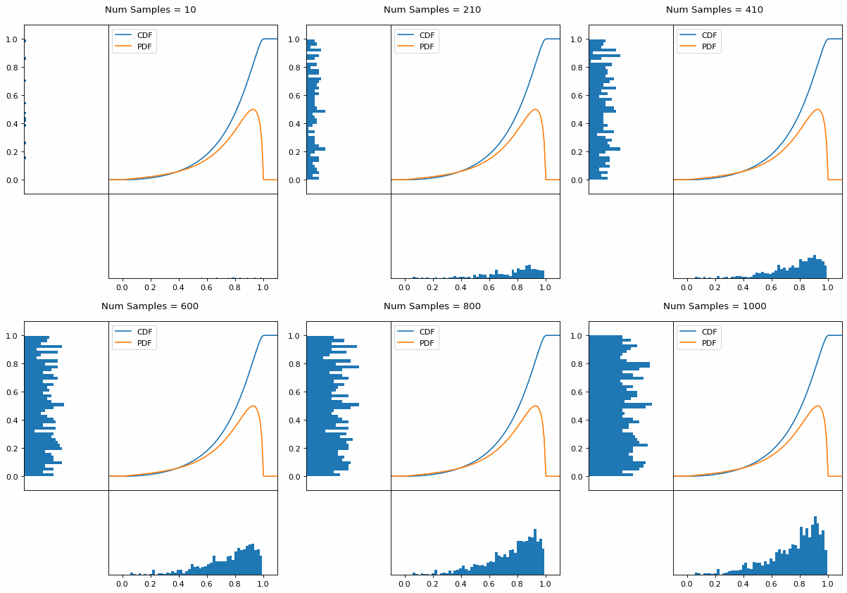
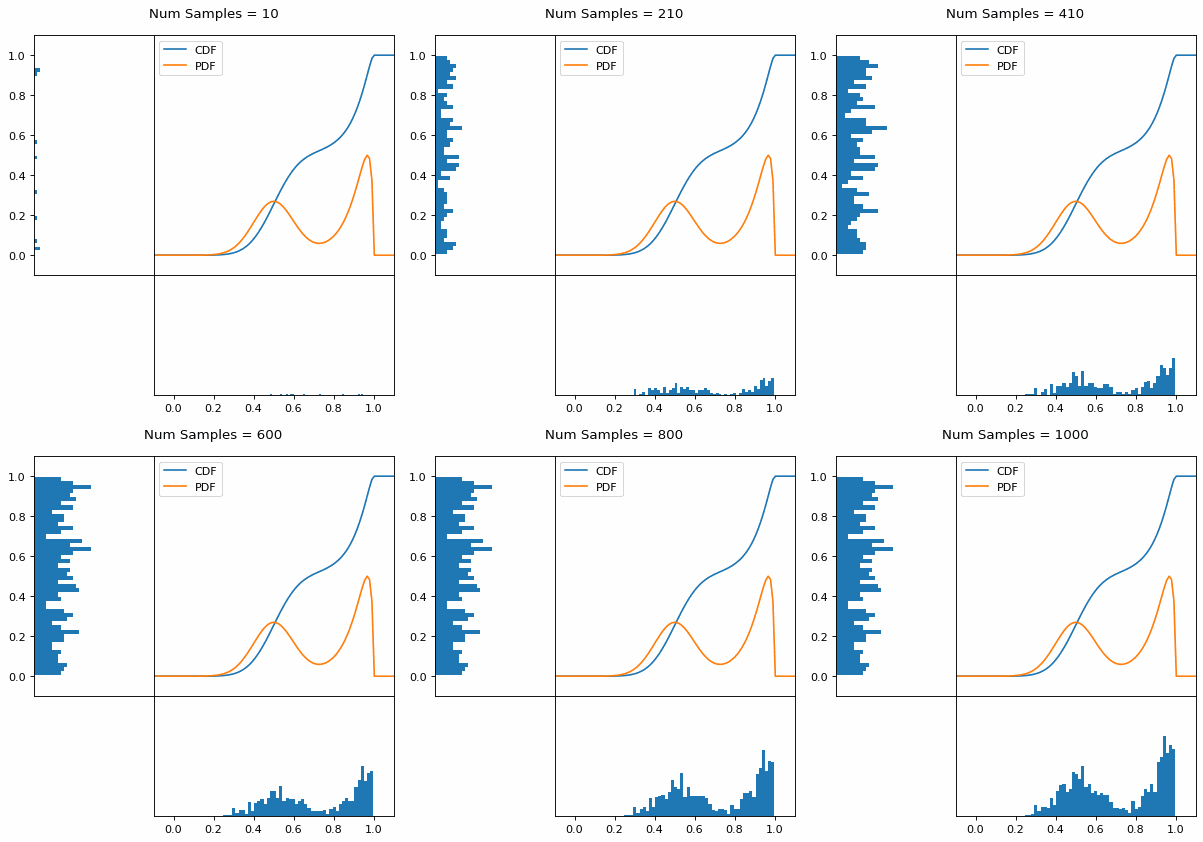
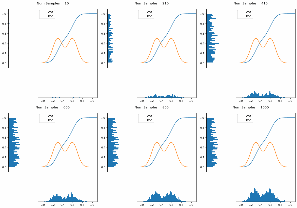
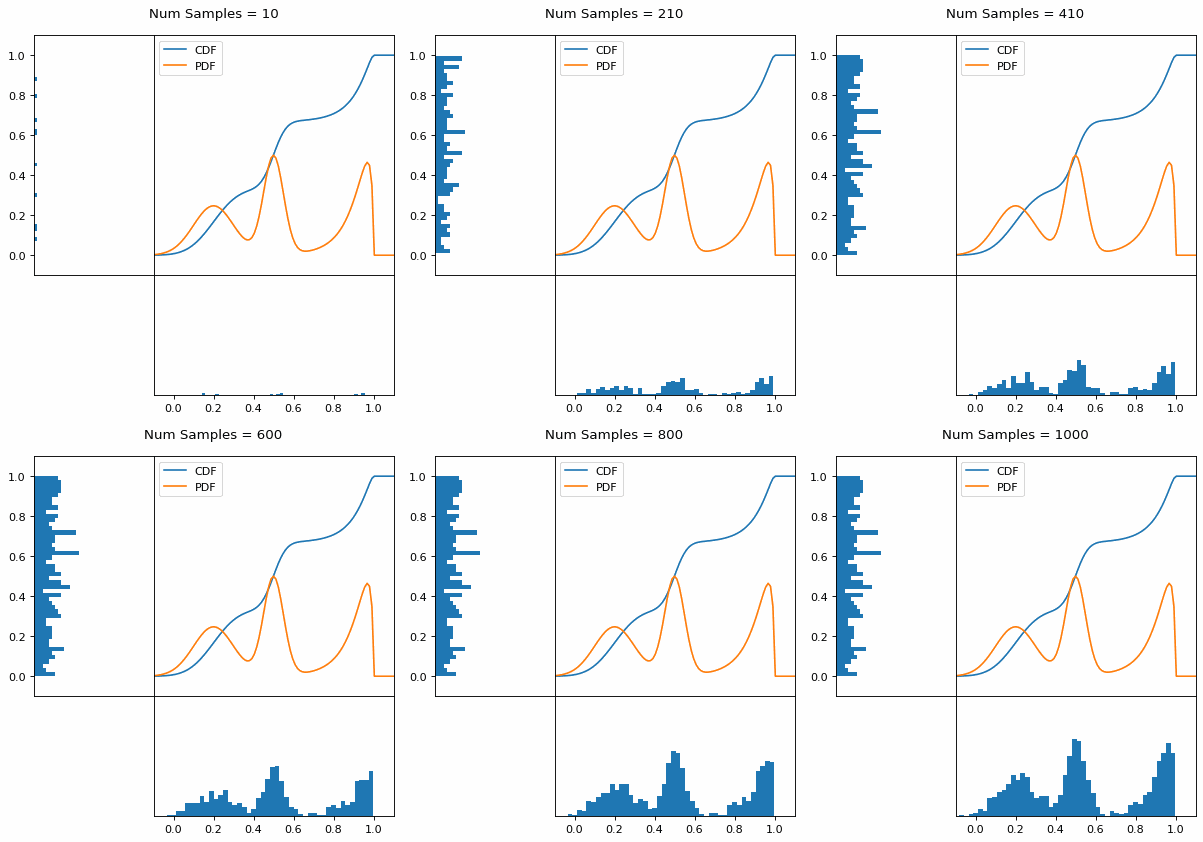
I always imagine the values on the left smashing into the cdf on the right and dropping wherever they hit. Bigger gradients in the cdf correspond to more samples in that area when the samples drop down.
The Math
So the question is, how is it that I can transform samples of the uniform distribution into samples of any probability distribution with an analytic cumulative distribution function?
As a test case, let’s say we want samples from the exponential distribution:
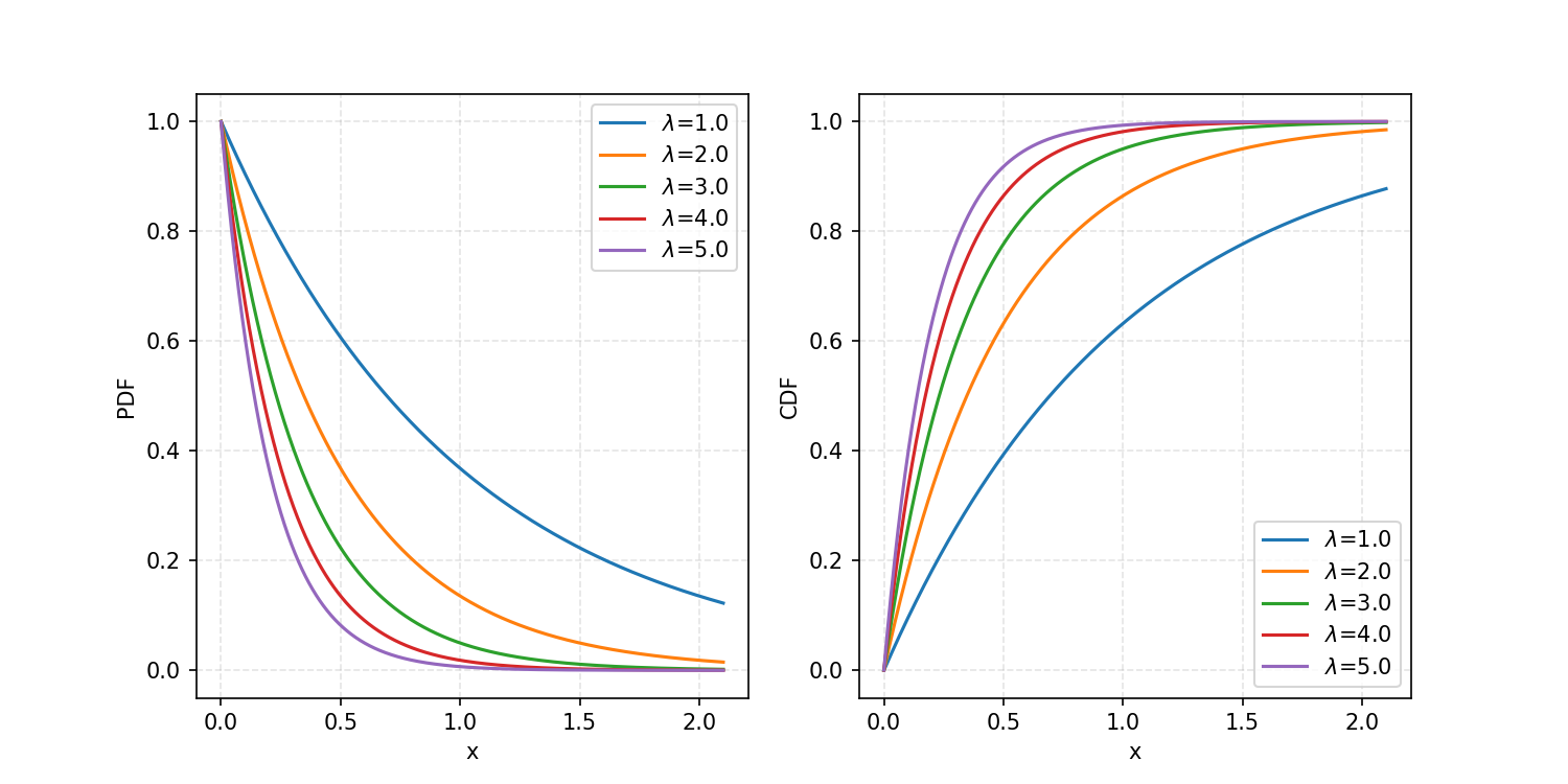
\[\begin{align} p(x) = \begin{cases} \exp(-\lambda x) & x \geq 0 \\ 0 & x < 0 \end{cases} \end{align}\]which we then integrate to specific $x$ values to get the CDF.
\[\begin{align} CDF(x) = \int_{-\infty}^{x} p(x') dx' = \begin{cases} 1-\exp(-\lambda x) & x \geq 0 \\ 0 & x < 0 \end{cases} \end{align}\]If I give a specific value of $x$ to the CDF, it will output the probability of being that value or below, for the given probability distribution. Here’s a plot showing some example curves.
And a reminder: our end goal is to produce some transformation \(T\)(spoiler: it’s the inverse CDF) that will transform uniformly distributed samples\(U\)into\(X\)where\(X\) follows whatever 1D probability density function we want.
\[\begin{align} T(U) = X \end{align}\]Cheating a little bit, we’re going to presume that this will involve the CDF.
By definition and our equation above:
\[\begin{align} CDF(x) = Prob(X\leq x) = Prob(T(U)\leq x) = Prob(U\leq T^{-1}(x)). \end{align}\]So what we’ve shown is that the CDF is equivalent to asking the probability that a uniform sample/value is less than or equal to \(T^{-1}(x)\). Well, here’s the cool bit: if I ask you
- what the probability of being less than or equal to 1? It’s 1. (As all the values/area in the distribution are equal to or less than 1.)
- what the probability of being less than or equal to 0? It’s 0. (As none of the values/area in the distribution are less than 0.)
- what the probability of being less than or equal to 0.5? It’s 0.5. (As half the values/area in the distribution are less than 0.5.)
And so on. So it follows that: \(\begin{align} CDF(x) = Prob(U\leq T^{-1}(x)) = T^{-1}(x). \end{align}\)
So you can clearly see that \(CDF = T^{-1}\) or equivalently \(T = CDF^{-1}\). And we have our transformation.
Coding up our own sampler
Now ritvikmath then goes on to solve for the exact analytical inverse of the exponential. It isn’t that hard, you can have a crack yourself, but what I’m interested in is: “if you give me a general probability density function, how can I sample it?” And let’s presume that either there is no closed-form expression for the inverse CDF or that I don’t have the time/can’t be bothered to figure it out.
Well, the inverse of a function is just if I give the inverse what were the outputs of the original function, then I should get what the inputs must have been. So if I can create a map (or an approximate map) of inputs to outputs, then just do the ol’ switcheroo, I can interpolate the result and get an approximate inverse CDF!
from scipy.interpolate import interp1d

def create_an_invcdf(pdf, inputs, kwargs):
    # We are implicitly presuming that the inputs are linearly spaced here and performing a finite Riemann sum
    pdf_outputs = pdf(inputs, **kwargs)

    cdf_outputs = np.cumsum(pdf_outputs)
    cdf_outputs /= np.max(cdf_outputs)

    inv_cdf_func = interp1d(y=inputs, x=cdf_outputs)

    return inv_cdf_func
I extract the pdf (a pmf would also work here) then calculate the cumulative sum, equivalent to a finite Riemann sum, dividing by the max value (which should be the last, but don’t worry) such that the cdf values range from \(\approx 0\) to 11.
Continuous Approx Case
We can then apply this to the exponential distribution we looked at previously, looking at values from 0 to 7.
u_inputs = np.linspace(0, 1, 1001)
x_inputs = np.linspace(0, 7, 1001)


def exact_exp_cdf_inverse(u, lam=1):
    return -np.log(1-u)/lam


# Plotting the results
fig, ax = plt.subplots(1, 2, figsize=(10, 5), dpi=150)

ax = np.array(ax).flatten()

for lambda_val in lambda_values:

    inv_cdf_func = create_an_invcdf(exp_func, x_inputs, {'lam':lambda_val})

    ax[0].plot(u_inputs, inv_cdf_func(u_inputs), label=r"$\lambda$="+f"{lambda_val}")


ax[0].set_ylabel(r"$CDF^{-1}$")
ax[0].set_xlabel("u")
ax[0].legend()
ax[0].grid(ls='--', c='grey', alpha=0.2)
ax[0].set_title("Approx")

for lambda_val in lambda_values:
    ax[1].plot(u_inputs, exact_exp_cdf_inverse(u_inputs, lam=lambda_val), label=r"$\lambda$="+f"{lambda_val}")

ax[1].set_ylabel("$CDF^{-1}$")
ax[1].set_xlabel("u")
ax[1].legend()
ax[1].grid(ls='--', c='grey', alpha=0.2)
ax[1].set_title("Exact")

plt.savefig("inv_cdf_comparison.png")
plt.show()
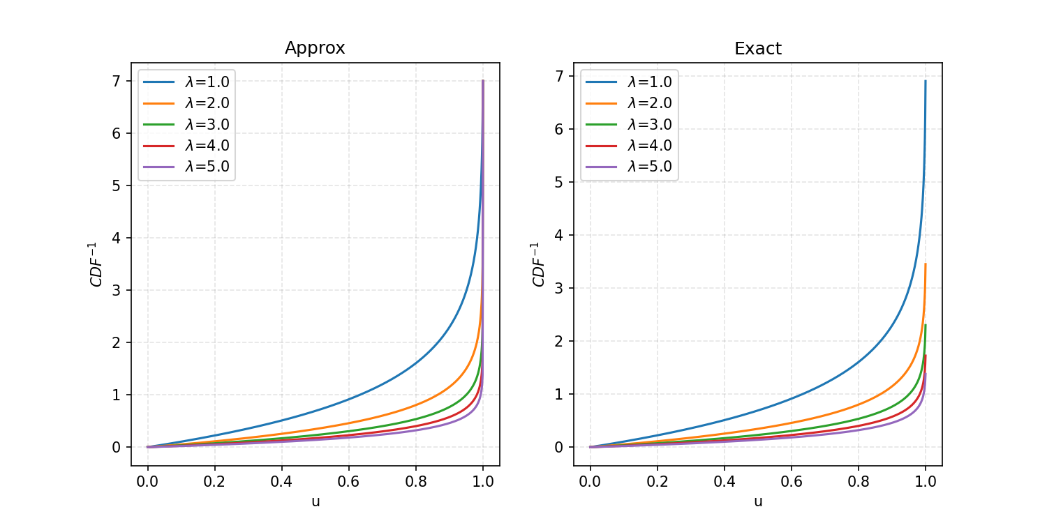
And then if we produce uniform random samples and feed them into these functions with lambda equal to 5, we get the following.
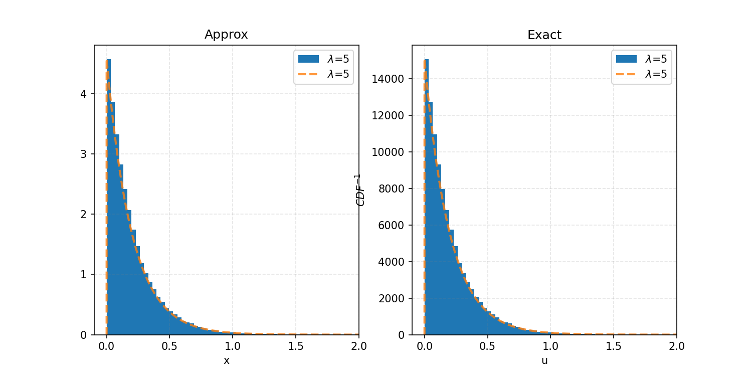
You can also see how you can immediately expand this to discrete distributions, except instead of an interpolation function, it would likely be better to use something like np.abs(input - cdf_outputs).argmin() to get the index of the exact input/output.
Next Steps
In my next post we’ll use this ability to sample “nice” probability distributions to sample “less nice” distributions using Rejection Sampling.
Presuming that we only sample in the range of the given inputs, we can think of this as the complete domain. The final value should correspond to one, hence the division. We could also take this step out if you are sure your distribution is properly normalized. ↩
